doi:10.4236/am.2011.25082 Published Online May 2011 (http://www.SciRP.org/journal/am)
A Problem of a Semi-Infinite Medium Subjected to
Exponential Heating Using a Dual-Phase-Lag
Thermoelastic Model
Ahmed Elsayed Abouelregal
Department of Mathematics, Faculty of Science, Mansoura University, Mansoura, Egypt E-mail: [email protected]
Received January 2, 2011; revised March 39, 2011; accepted April 2, 2011
Abstract
The problem of a semi-infinite medium subjected to thermal shock on its plane boundary is solved in the context of the dual-phase-lag thermoelastic model. The expressions for temperature, displacement and stress are presented. The governing equations are expressed in Laplace transform domain and solved in that do-main. The solution of the problem in the physical domain is obtained by using a numerical method for the inversion of the Laplace transforms based on Fourier series expansions. The numerical estimates of the dis-placement, temperature, stress and strain are obtained for a hypothetical material. The results obtained are presented graphically to show the effect phase-lag of the heat flux q and a phase-lag of temperature
gra-dient on displacement, temperature, stress.
Keywords: Generalized Thermoelasticity, Dual-Phase-Lag Model, Semi-Infinite Medium, Laplace Transform
1. Introduction
Biot [1] (1956) introduced the theory of coupled ther-moelasticity to overcome the first shortcoming in the classical uncoupled theory of thermoelasticity where it predicts two phenomena not compatible with physical observations. First, the equation of heat conduction of this theory does not contain any elastic terms. Second, the heat equation is of a parabolic type, predicting infi-nite speeds of propagation for heat waves. The governing equations for Biot theory are coupled, eliminating the first paradox of the classical theory. However, both theo-ries share the second shortcoming since the heat equation for the coupled theory is also parabolic.
Thermoelasticity theories that predict a finite speed for the propagation of thermal signals have aroused much interest in the last three decades. These theories are known as generalized therrnoelasticity theories. The first generalizations of the thermoelasticity theory is due to Lord and Shulman [2] who introduced the theory of gen-eralized thermoelasticity with one relaxation time by po- stulating a new law of heat conduction to replace the classical Fourier’ law. This law contains the heat flux vector as well as its time derivative. It contains also a
new constant that acts as a relaxation time. The heat equ- ation of this theory is of the wave-type, ensuring finite speeds of propagation for heat and elastic waves. The re- maining governing equations for this theory, namely, the equations of motion and the constitutive relations remain the same as those for the coupled and the uncoupled theories. This theory was extended by Dhaliwal and She-rief [3] to general anisotropic media in the presence of heat sources.
A generalization of this inequality was proposed by Green and Laws [4] Green and Lindsay obtained another version of the constitutive equations in [5]. The theory of thermoelasticity without energy dissipation is another ge- neralized theory and was formulated by Green and Na-ghdi [6]. It includes the thermal displacement gradient among its independent constitutive variables, and differs from the previous theories in that it does not accommo-date dissipation of thermal energy.
effect on the behavior of heat transfer. The physical meanings and the applicability of the DPL mode have been supported by the experimental results [9]. The dual-phase-lag (DPL) proposed by Tzou [9] is such a modification of the classical thermoelastic model in which the Fourier law is replaced by an approximation to a modified Fourier law with tow different time transla- tions: a phase-lag of the heat flux qand a phase-lag of temperature gradient . A Taylor series approximation of the modified Fourier law, together with the remaining field equations leads to a complete system of equations describing a dual-phase-lag thermoelastic model. The model transmits thermoelastic disturbance in a wave-like manner if the approximation is linear with respect to
q
and , and 0 ≤ < q; or quadratic in q and
linear in , with q> 0 and > 0. This theory is
developed in a rational way to produce a fully consistent theory which is able to incorporate thermal pulse trans-mission in a very logical manner.
Danilovskaya [10] was the first to solve an actual problem in the theory of elasticity with nonuniform heat. The problem was for a half-space subjected to a thermal shock in the context of what became known as the theory of uncoupled thermoelasticity. Chandrasekharaiah and Srinath [11] studied the one dimensional thermal wave propagation in a half space based on the theory of ther-moelasticity without energy dissipation due to a constant step in temperature applied to the boundary. Roychoud-huri and Dutta [12] studied thermoelastic interactions in an isotropic homogeneous thermoelastic solid containing time-dependent distributed heat sources which vary pe-riodically for a finite time interval in the context of Green and Naghdi theory. Sherief and Dhaliwal [13] solved a generalized one-dimensional thermal-shock problem for small times. Allam et al. [14] discussed magneto-thermoelasticity for an infinite body with a spherical cavity and variable material properties without energy dissipation.
The present paper is organized as follows. Section 2 describes the formulation of the problem and the gov-erning equations. Section 3 discusses the Laplace trans- form technique and the solution in the transformed do-main is obtained using a potential function. Section 4 summarizes the inverse Laplace transforms using a nu-merical method based on Fourier expansion techniques. The last section is devoted to the numerical example for finding the temperature, displacement and the stress. These distributions are also depicted graphical.
2. Formulation of the Problem
We shall consider a homogeneous, isotropic, thermoelas-tic solid, occupying the region x0 where the
x
-axisis taken perpendicular to the bounding plane of the half- space pointing inwards. The boundary conditions for tem-perature is in the form of exponential heating, a more realistic situation. It is assumed that the state of the me-dium depends only on x and t and that the displace-ment vector has components
u x
, , 0, 0t
.The equation of motion in the absence of body forces in the one dimensional case has the form
2 2
2 2
u
2
u T
x
t x
(1)
The constitutive equation will take the following form
xx= +2 T
u x
(2)
The Chandrasekharaiah and Tzou theory is such a mo- dified of classical thermoelasticity model in which the Fourier law is replaced by an approximation of the equa-tion
q
q x t, KT x t,
(*) The model transmits thermoelastic disturbances in a wave-like manner if Equation (*) is approximated by1 q q K 1 T
t t ,
where 0 q.
Hence, we get the heat conduction equation in the context of dual-phase-lag model in the form
2 2
0 2
1 1 q E
T T
K C
t x t t
u T
x t
(3)
where xx is the stress, and are the Lamé
con-stants, is equal to
32
t, t is the thermalexpansion coefficient, K is the thermal conductivity,
E
C is the specific heat per unit mass at constant strain, ρ is the density of the medium and is the heat flux
vector. i
q
Moreover, if we put = 0 and q= τ (the first
re-laxation time), fundamental equations possible for the Lord and Shulman's theory.
The initial and boundary conditions are taken as
, 0
, 0, 0t
u x t
u x t x
t
0
t
0
0
,
, t 0
t
T x t
T x t x
t
, 0,
/0
/0
0 0
0
,
, et , 1 e t
x
x
u x t
T x t T
x
(4)
where 0 is constant and the regularity boundary
1 ,
For convenience, we shall use the following non-di-mensional variables
2
1 1
' , ' , '
x c x u c u t c t
2 2
1 1 0 1
' , ' , '
q q
t c t c t c2
0,
0
' , ' xx,
xx T T T where 1 2 , E C c K
In terms of these variables, Equations (1)-(3) become (where the primes are suppressed for simplicity)
2 2
2 2 .
u u a T
x
t x
(5)
2 2
2
1 1 q
T T
t t g
t x t t
u x t
(6)
2 xx= u bT x
(7)
where 2 0 0 2 1 2 , , , . E T T
a b g
C c
and initial and boundary conditions will be
0
0
,
, t 0
t
u x t
u x t x
t
, 0,
0
0 ,
, 0
t
t
T x t
T x t x
t
, 0,
/0
0
0
,
, e t t , 1 e t t
x
x
u x t T x t
x 0 /
(8)
3. Solution in the Laplace Transform
Domain
We use the Laplace transform of both sides of the last equations which is defined in the form
0
e st d.
f s f t
tHence, we obtain Equations (5-7) in the form
2 2 2 d , d d T
s u ad
x x
(9)
22
d
1 1 1
d
d q q
t s s t s T s t s g
2 xx d = d u bT x
(11)
where the over bar symbol denotes its Laplace transform and s denotes the Laplace transform parameter.
The boundary conditions (8) in the Laplace transform can be expressed in the form
0 0 0 0 0 0 , , 1 d , . d 1 x x t T x tst
u x t t
x s st
(12)
Introducing the thermoelastic potential function defined by the relation
d d u
x
(13)
Equations (9-10) reduce to
2 2 2 d
,
dx s aT
(14)
1
d22
1
1
d22d q q d
t s s t s T s t s g .
x x
(15)
Eliminating from Equations (14) and (15), we ob-tain T
4 2 2 2 4 2d 1 d 0
dx s P dx s P
,
(16)
where is the mechanical coupling constant defined by ag and
1 1
q
s t s
P
t s
.
The solutions of Equation (16) bounded at infinity can be written in the form:
1
1e 2e
m
A A
m2 (17)
where A1 and A2 are parameters depending on s to be
determined from the boundary conditions, m1and 2
are the roots with positive real parts of the characteristic equation
m
4 2 1 2 2 0
m s P m s P (18)
1
m and m2 are given by
22 2 1,2 1 1 2 2 4
s P s P
m s P
(19) du x x
(10)
The expression for displacement and temperature can be written in the forms
1
1 1e 2 2
m
1
22 2 2 2
1 2
1e m 2e m
m s m s
T A
a a
A
(21) (21)
Substituting from Equations (20) and (21) into Equa-tion (11), we obtain
Substituting from Equations (20) and (21) into Equa-tion (11), we obtain
1
2 2
2 2
1 1
2
2 2
2 2
e
e m xx
m
b bs
m A
a a
b bs
m A
a a
(22)
From the boundary conditions (12), it follows that
2 2
2 0
1 3 2
0 1 2
1 1
m st s
A
s st m m
2 ,
2 2
1 0
2 3 2
0 1 2
1 1
m st s
A
s st m m
2
4. Numerical Inversion of the Laplace
Transform
In order to determine the conductive and thermal tem-perature, displacement and stress distributions in the time domain, we adopt a numerical inversion method based on a Fourier series expansion [15]. In this method, the inverse g(t) of the Laplace transform g(s) is approxi-mated by the relation
/11 1
1 1
Re ,0 ,
2
ct N
ikt t
k g c
e ik
g t e g c t
t t
t(23) where Re is the real part and i 1 is imaginary number unit and is a sufficiently large integer rep-resenting the number of terms in the truncated infinite Fourier series. For faster convergence, numerous nu-merical experiments have shown that the value of c satisfies the relation Tzou [9].
N
4.7 ct N must chosen such that
1 /
1 1 e Re ect ikt t g c ik
t
(24)
where 1 is a persecuted small positive number that
corresponds to the degree of accuracy to be achieved. The parameter c is a positive free parameter that must be greater than the real parts of all singularities of g s
. The optimal choice of c was obtained according to the criteria described in [15].Formula (23) was used to invert the Laplace trans-forms in Equations (20)-(22), given the temperature, stress, and displacement distributions.
5. Numerical Results
Now, we will consider a numerical example for which computational results are given. For this purpose, Copper is taken as the thermoelastic material for which we take the following values of the different physical constants [16]
368
K , 1.78 105,
t
383.1,
E
C g 1.61,
10 10
= 8954, =7.76 10 , =3.86 10 ,
2 0
= 8886.73, =4, T =293, =0.0168
.
The non-dimensional temperature T , displacement , and stress component
u xx distributions were
evalu-ated on the x-axis. Further by setting the phase-lag of the heat flux t to zero, the results due to the Lord and
Shulman's theory are obtained. The computations were carried out for one value of time, namely for t0.1.
The graphs of the temperature, displacement and thermal stress due to phase-lag of the heat flux tqare
exhibited graphically in Figures 1-3. The results carried
0 0.005 0.01 0.015 0.02 0.025 0.03
0 0.2 0.4 0.6 0.8 1
D
isp
lacem
en
t
0.05
q
t
0.1
q
t
0.2
q
[image:4.595.310.530.347.501.2]t
Figure 1. Displacement vs. distance for different values of phaselag of the heatflux.
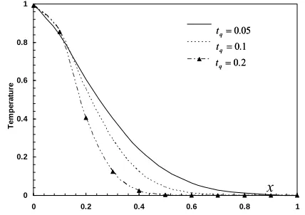
0 0.2 0.4 0.6 0.8 1
0 0.2 0.4 0.6 0.8 1
Te
m
p
e
ra
tu
re
0.05
q
t
0.1
q
t
0.2
q
t
x
0.05
q
t
0.1
q
t
0.2
q
t
x
x
[image:4.595.321.535.545.696.2]-0.6 -0.4 -0.2 0
0 0.2 0.4 0.6 0.8 1
T
h
er
m
al
S
tr
e
ss
x
0.05
q
t
0.1
q
t
0.2
q
[image:5.595.63.285.78.241.2]t
Figure 3. Thermal stress vs. distance for different values of phaselag of heatflux.
out for three values of tq, namely tq=0.05, 0.1 and 0.2. We can deduce that:
1) The parameter has significant effects on all the
fields. q
t
2) The wave has a finite speed of propagation. This result shows that the DPL model agree with the general-ized thermoelasticity.
3) The temperature and displacement starts with its maximum value at the origin and decreases until attain-ing zero beyond a wave front for the generalized theory, which agree with the boundary conditions.
4) The magnitude of the stress increases rapidly as x increases and it attains a peak value at , thereaf-ter it decreases slowly with increasing
= 0.1 x
x whereas the magnitude of the peak value is reduced with the increase oftq.
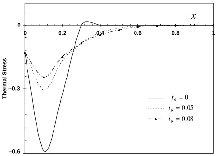
Figures 4-6 show the heat, the displacement, and the stress respectively with distance x at the same instance with different values of the phase-lag of tem-perature gradient parameter
0.1 t
0 q
t t t0.05 t
which means coupled thermoelasticity model of Biot, which means generalized thermoelasticity model of Lord and Shul-man and for (t and ) means
that DPL model and we found that, the parameter
0 t
0.08 0
t
t
has a significant effects on all the fields.
In all these figures, it is clear that the values of solu-tions for L-S theory are large in comparison with those for DPL model. This may be due to the nature of the boundary conditions, which we take.
6. Conclusions
In the framework of this article, a problem of a half- space whose surface is rigidly fixed and subjected to the effects of a thermal shock on the surface within the con-text of the theory of generalized thermoelasticity pro-
0 0.005 0.01 0.015 0.02 0.025 0.03
0 0.2 0.4 0.6 0.8 1
Di
s
p
la
c
e
m
e
n
t
0
t
0.05
t
0.08
t
x
–0.2
–0.4
[image:5.595.310.535.80.251.2]–0.6
Figure 4. Displacement vs. distance for different values of phaselag of gradient of temperature.
-0.1 0.1 0.3 0.5 0.7 0.9 1.1
0 0.2 0.4 0.6 0.8 1
T
e
m
p
er
atu
re
0
t
0.05
t
0.08
t
x
–0.1
Figure 5. Temperature vs. distance for different values of phaselag of gradient of temperature.
-0.6 0
0 0.2 0.4 0.6 0.8 1
l S
tr
e
s
s
0
t
0.05
t
0.08
t
x
Th
e
rm
a
-0.3
–0.3
–0.6
Figure 6. Thermal stress vs. distance for different values of phaselag of gradient of temperature.
posed by Tzou.
According to the above results, we can conclude that: 1) As the phase-lag of the heat flux qconstant
[image:5.595.314.533.289.439.2] [image:5.595.313.534.476.635.2]displacement and stress decrease.
2) The increases of the phase-lag of gradient of tem-perature t decrease the components of temperature, displacement and stress distributions.
3) We found that, the parameters and tq t have
significant effects on all the fields.
4) The phenomenon of finite speeds of propagation is manifested in all these figures.
The comparison of different theories of thermoelastic-ity, i.e. Lord and Shulman theory and Chandrasekharaiah and Tzou model is carried out.
7. References
[1] M. Biot, “Thermoelasticity and Irreversible Thermody-Namics,” Journal of Applied Physics, Vol. 27, No. 3, 1956, pp. 240-253.doi:10.1063/1.1722351
[2] H. Lord and Y. Shulman, “A Generalized Dynamical Theory of Thermoelasticity,” Journal of the Mechanics and Physics of Solids, Vol. 15, No. 5, 1967, pp. 299-309. doi:10.1016/0022-5096(67)90024-5
[3] R. Dhaliwal and H. Sherief, “Generalized Thermoelastic-ity for Anisotropic Media,” Quarterly of Applied Mathe-matics, Vol. 33, 1980, pp. l-8.
[4] A. E. Green and N. Laws, “On the Entropy Production Inequality,” Archive for Rational Mechanics and Analysis, Vol. 45, No. 1, 1972, pp. 47-53.doi:10.1007/BF00253395 [5] A. E. Green and K. A. Lindsay, “Thermoelasticity,”
Journal of Elasticity, Vol. 2, No. 1, 1972, pp. 1-7. doi:10.1007/BF00045689
[6] A. E. Green and P. M. Naghdi, “Thermoelasticity With-out Energy Dissipation,” Journal of Elasticity, Vol. 31, No. 3, 1993, pp. 189-208.doi:10.1007/BF00044969 [7] D. Y. Tzou, “Macro- to Microscale Heat Transfer: The
Lagging Behavior,” 1st Edition, Taylor & Francis, Wa- shington, 1996.
[8] D. Y. Tzou, “A Unified Approach for Heat Conduction
From Macro- to Micro- Scales,” Journal of Heat Transfer, Vol. 117, No. 1, 1995, pp. 8-16.doi:10.1115/1.2822329 [9] D. Y. Tzou, “Experimental Support for the Lagging
Be-havior in Heat Propagation,” Journal of Thermophysics and Heat Transfer, Vol. 9, 1995, pp. 686-693.
doi:10.2514/3.725
[10] V. Danilovskaya, “Thermal Stresses in an Elastic Half- space Due to Sudden Heating of Its Boundary,” Prikl Mat. Mekh., In Russian, Vol. 14, 1950, pp. 316-324.
[11] D. S. Chandrasekharaiah and K. S. Srinath, “One-Dimen- sional Waves in a Thermoelastic Half-Space Without En-ergy Dissipation,” International Journal of Engineering Science, Vol. 34, No. 13, 1996, pp. 1447-1455.
doi:10.1016/0020-7225(96)00034-1
[12] S. K. Roychoudhuri and P. S. Dutta, “Thermoelastic In-teraction Without Energy Dissipation in an Infinite Solid with Distributed Periodically Varying Heat Sources,” In-ternational Journal of Solids Structures, Vol. 42, 2005, pp. 4192-4203.
[13] H. Sherief, and R. Dhaliwal, “Generalized One-Dimen- sional Thermal Shock Problem for Small Times,” Journal of Thermal Stresses, Vol. 4, No. 3-4, 1981, pp. 407-420. doi:10.1080/01495738108909976
[14] M. N. Allam, K. A. Elsibai and A. E. Abouelregal, “Magneto-Thermoelasticity for an Infinite Body with a Spherical Cavity and Variable Material Properties With-out Energy Dissipation,” International Journal of Solids and Structures, Vol. 47, No. 20, 2010, pp. 2631-2638. doi:10.1016/j.ijsolstr.2010.04.021
[15] G. Honig and U. Hirdes, “A Method for the Numerical Inversion of the Laplace Transform,” Journal of Compu-tational and Applied Mathematics, Vol. 10, No. 1, 1984, pp. 113-132.doi:10.1016/0377-0427(84)90075-X [16] H. Youssef, “Thermomechanical Shock Problem of