Sebastian Kosmeier, Svetlana Zolotovskaya, Kishan Dholakia, and Michael Mazilu
SUPA, School of Physics and Astronomy, University of St Andrews, North Haugh, KY16 9SS, St Andrews, UK
Anna Chiara De Luca
Institute of Protein Biochemistry, National Research Council, Via P. Castellino 111, 80313, Naples , Italy and To whom correspondence should be addressed; [email protected]
Andrew Riches
School of Medicine, University of St Andrews, North Haugh, KY16 9TF, St Andrews, UK
C. Simon Herrington
Medical Research Institute, University of Dundee,
Ninewells Hospital Medical School, James Arrott Drive, DD1 9SY, Dundee, UK (Dated: 17 October 2014)
Various forms of imaging schemes have emerged over the last decade that are based on correlating variations in incident illuminating light fields to the outputs of single ‘bucket’ detectors. However, to date, the role of the orthogonality of the illumination fields has largely been overlooked and furthermore, the field has not progressed beyond bright field imaging. By exploiting the concept of orthogonal illuminating fields, we demonstrate the application of optical eigenmodes (OEi) to wide field, scan-free spontaneous Raman imaging, which is notoriously slow in wide-field mode. The OEi approach enables a form of indirect imaging that exploits both phase and amplitude in image reconstruction. The use of orthogonality enables us to non-redundantly illuminate the sample and, in particular, use a subset of illuminating modes to obtain the majority of information from the sample, thus minimising any photobleaching or damage of the sample. The crucial incorporation of phase, in addition to amplitude, in the imaging process significantly reduces background noise and results in an improved SNR for the image while reducing the number of illuminations. As an example we can reconstruct images of a surface-enhanced Raman spectroscopy (SERS) active sample with approximately an order of magnitude fewer acquisitions. This generic approach may readily be applied to other imaging modalities such as fluorescence microscopy or nonlinear vibrational microscopy.
I. INTRODUCTION
A generic challenge in all forms of imaging is to acquire information in a rapid, damage-free manner. In the op-tical domain, photo-damage can be an issue in numerous forms of biomedical methods and furthermore the very manner of sample illumination is typically non-optimal. In this context, structured illumination aims to engineer the excitation/illumination beams to achieve either faster acquisition [1], higher resolution [2, 3] or even 3D imaging capabilities [4]. Structured illumination in combination with ‘bucket’ detection (single detector acquisition) has gained popularity due to its inherent simplicity. Sepa-rately, illumination based upon non-redundant imaging relies on the use of structured light fields incident on a sample to detect its features by using the smallest num-ber of illuminations i.e. to achieve the fastest acquisi-tion. This is normally not the case when considering a scanned Gaussian beam approach where the partial overlap between adjacent excitation spots leads to no additional information (‘redundant’ measure) and to a decreased image resolution. Due to their orthogonality, optical eigenmodes (OEi) offer a natural set of fields that avoid any overlap in the probing the optical degrees of
freedom of the sample [5, 6]. Additionally, the experi-mental in situ determination of the optical eigenmodes has the advantage of automatically taking into account all optical aberrations present in the optical system. It is therefore advantageous to use these OEi as structured illumination fields in the context of imaging.
Previously, we have developed a coherent indirect imaging technique [7] based on OEi fields. This paper demonstrates the first experimental application of this approach to the case of imaging spontaneous Raman scat-tering. In particular, Raman scattering is a vibrational microscopy method offering a label-free imaging contrast mechanism capable of probing non-invasively the chemi-cal composition of biologichemi-cal and inert materials at micro-scopic scales [8–12]. It has promise for many applications yet has been hampered by long acquisition times which in turn has resulted in researchers resorting typically to more complex nonlinear vibrational spectroscopy meth-ods.
suitable for rapid large-scale imaging of pharmaceutical tablets as an example. Various Raman imaging method-ologies have been proposed to alleviate this issue. In point and line scanning Raman imaging [13, 14, 20, 21] a circular or line shaped laser spot raster scans the sam-ple in two spatial dimensions with a Raman spectrum recorded at each position.
Other direct imaging techniques illuminate the sam-ple using a number of laser spots or a wide-field laser beam. The resulting Raman signal is directly imaged on a filtered detector acquiring a single measurement. For example in [22], the authors used an Hadamard mask to produce structure illumination pattern on the sam-ple to genarate only one-dimensional compressed Raman image. Additional wide-field Raman approaches include tuneable detection band-pass filters and two-dimensional detector [23–25]. However, this method discards the Raman scattered photons outside the wavelength detec-tion band rendering this approach spectrally inefficient. Recently, a multivariate hyperspectral Raman imaging (MHRI) approach has been introduced by Davis et al. based on a compressive spectral detection strategy [26]. Our approach applies a non-redundant approach to the illumination side of the Raman imaging enabling a step change in the acquisition process for this modality. This non-redundant approach is equivalent to a compression in the number of measures when comparing to a stan-dard raster scan method. This is due to the fact that the standard raster scan approach inherently leads to an overlap between adjacent optical beams.
In our non-redundant Raman OEi imaging, we illumi-nate the sample with a predetermined set of optical eigen-modes. For each of the illuminations used, we measure the Raman spectrum from which we subsequently recon-struct the hyperspectral Raman image of the sample. An important outcome of this method is the adaptive reso-lution that can be achieved. Indeed, to increase the res-olution, we do not need to rescan the sample with a finer step size but simply continue to probe the sample with increasingly higher order OEi illuminations. In effect, the higher the order of the OEi illumination, the finer the de-tails probed by the OEi illumination. Furthermore, due to the non-redundant nature of OEi based structured il-lumination, we realise a given imaging resolution using
correspond to a non-redundant set of orthogonal optical eigenmode beam profiles.
II. RESULTS
a. Determining the OEi. Figure 1a describes our ex-perimental set-up. Figure 1b shows the theoretical spa-tial field distribution of the first nine Optical Eigenmodes
Eℓin the region of interest (ROI) [7, 30]. We observe that as the order of the modeℓincreases finer details are ac-cessed. In order to check the orthonormality relation, in the region of interest (ROI), ∫ROIEkE∗ldσ = δkl of the experimentally implemented OEi, the complex prod-uctEkE∗l is determined from four intensity acquisitions according to the polarization identity [31]. Each entry in the matrix in Fig. 1c corresponds to an orthonormal-ity relation for a pair k, l. The matrix is almost diago-nal, hence demonstrating orthonormality of the experi-mentally implemented modes in good approximation (for more details see the Methods section). Remark that the presence of high aberrations precludes the use of the-oretically calculated eigenmodes, however, in this case these eigenmodes can be experimentally determined [5] automatically accounting for any aberration and angular dependance.
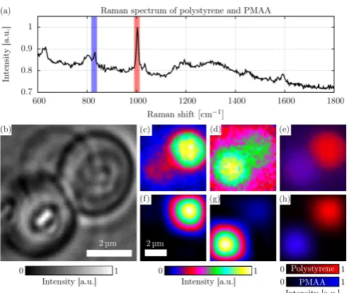
b. Raman OEi imaging. As a first example, we im-aged a sample consisting of a polystyrene bead in the top right corner of the ROI and a PMAA bead in the lower left corner, both beads are 3µm in diameter. Fig-ure 2b shows a brightfield image of the sample. FigFig-ures 2c and 2d depict raster scan Raman images of the sample obtained by integrating the main polystyrene and PMAA peaks, respectively (shown in Fig. 2a). In Fig. 2e the in-formation from Fig. 2c and Fig. 2d are superimposed in a hyperspectral image, highlighting the polystyrene bead (red color) and the PMAA bead (in blue).
hy-FIG. 1. (a) Experimental configuration for Optical Eigen-mode Raman microscopy. LLF: Laser line filter at 785 nm; L: Lens; SLM: Spatial light modulator; M: Mirror; I: Iris to filter out first diffraction order from SLM; DBS: Dichroic beam splitter reflecting visible light and transmitting infrared light; CCD: CCD camera; NF: Notch filters to transmit Ra-man scattered light into the spectrograph; MO: Microscope objective; S: Sample. (b) Spatial field distribution and (c) orthogonality matrix of the first nine OEi.
[image:3.595.314.563.52.222.2]FIG. 2. (a) Spectrum for one polystyrene bead and one PMAA bead illuminated with the 4th eigenmode and 3 s ac-quisition time. The area of the PMAA peak is indicated in blue while that of polystyrene is highlighted in red. (b) White-light image of the sample with a polystyrene bead in the top right corner and a PMAA bead in the lower left corner. (c), (d) Raman images obtained with 26×26 points raster scans. (f), (g) OEi Raman images corresponding to (c) and (d). (e) Graphical superposition of the intensity distributions in (c) and (d), showing the positions of the polystyrene bead (red) and the PMAA bead (blue). (h) The same as (e) for the OEi images.
FIG. 3. (a) Schematic of the SERS sample: 200 nm gold particle on a gold surface coated with the analyte dithiol. The hotspot between the gold layer and the sphere gives rise to a SERS signal. (b) SEM image of a sample area similar to the imaged one. (c) Reflected laser light from the 9μm×9μm ROI chosen for imaging. Two agglomerates of gold particles are visible as dark spots. (d) SERS Raman raster scan of the sample plane. (e-i) OEi imaging reconstruction forM = 4 to M= 60 modes. (j) SERS spectrum of dithiol.
FIG. 4. (a) Experimental signal to noise ratio (SNR) and noise level as a function on the number of OEi illuminations. (b) Theoretical SNR and noise level as a function on the num-ber of OEi illuminations for a system paraxial optical stochas-tically system including CCD readout, SLM beam creation and optical system noise.
perspectral Raman OEi image. Both beads are clearly re-constructed in agreement with the standard raster scans, hence demonstrating the functionality of the method and its non-redundant nature. Furthermore, we remark that the OEi images visually exhibit a lower background noise compared to the raster scans.
[image:3.595.313.558.350.439.2] [image:3.595.52.299.355.562.2]the gold particle agglomerates. The corresponding OEi based images are depicted in Figs. 3e to 3i for projection ofM = 4 toM = 60 modes.
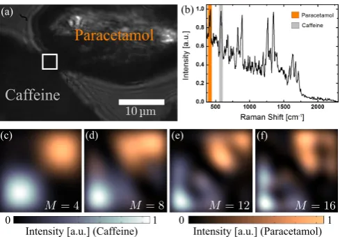
d. Signal to noise ratio. In Fig. 3, we observe vi-sually that increasing the number M of OEi used, the location and size of the SERS hotspots is reproduced with more accuracy. This effect can be quantified exper-imentally Fig. 4a and theoretically Fig. 4b by measuring the changes in the SNR and noise level as a function of the number of OEi illuminations used. The SNR is defined as the ratio between maximum Raman peak, in the high signal region, and the average signal from the image region void of Raman active medium where any measured signal can be associated with system noise. To determine the experimental SNR, we used the maximum Raman peak of the image divided by the mean value in the dotted squares in Figs. 3d,i for the raster scan and for the OEi image respectively. Note that, by adjusting the exposure time for each acquisition accordingly, the total laser power used to obtain both methods was identical. The results from the numerical simulation presented in Fig. 4b illustrate the case of a paraxial optical system consisting of a phase and amplitude mask for the SLM, an apertured lens modelling a generic finite optical sys-tem and the imaging plane corresponding to the Fourier plane with respect to the SLM plane. The model takes into account noise in the system (beam pointing stability and detection) for both the determination and the sub-sequent use of the OEi for imaging. Multiple numerical realisations are shown to visualise the effect of the noise. e. Pharmaceutical applications. Finally, the appli-cability of the Raman OEi imaging was investigated in a pharmaceutical context. In particular, the compound distribution of the well-known anticongestion and anal-gesic compound SUDAFED (Wrafton Laboratories Ltd) was determined. Each capsule contains a microcrystal mixture of paracetamol (500 mg), caffeine (25 mg), and phenylephrine hydrochloride (6.1 mg). A white-light full field image of the sample is shown in Fig. 5a. The ROI of 3.6×3.6μm, marked with the white square, includes two adjacent microcrystals. Fig. 5b shows a typical Raman spectrum of the two compounds illuminated simultane-ously byℓ= 12 OEi. The reconstructions, based on the coupling coefficients of the Raman bands unique for each
FIG. 5. (a) Full field of view image of a SUDAFED sample: A paracetamol crystal (top right corner) and a caffeine crystal (bottom left corner). The white square indicates the ROI. (b) Spectrum of the compound sample, in the ROI, illuminated with the 12th OEi mode, 5 s acquisition time and 250μm slit width. (c-f) Hyperspectral images of the ROI for different numberM of OEis.
compound, are depicted in Figs. 5c to 5f forM = 4 to
M = 16 modes. It can be seen that two substances are clearly resolved.
III. DISCUSSION
[image:4.595.316.561.49.219.2]plane using a holographic approach [34] as opposed to the polarization identity [31].
A further advantage of the method presented here is the improvement in the signal to noise ratio (SNR). If we look at the SERS experimental data (Fig. 3), forM = 60 modes good visual agreement of the OEi image (Fig. 3i) and the reference image (Fig. 3c) is observed. As for the images of the beads, the OEi images of the SERS sample exhibit a lower background than the raster scans. This visual impression was confirmed quantitatively in terms of the SNR (see Fig. 4a). With a value of 17.7, the SNR in the raster scan is an order of magnitude lower com-pared to the value of 245 measured in the OEi image. Fig. 4a also shows that increasing the number of OEi illuminations implies an increase of the SNR. A max-imum (in this case at M = 35) is achieved when the noise level drops below a certain measurement resolution threshold (determined by considering the readout noise of the detector and its dynamic range). Additionally, each OEi mode is associated with a optical coupling efficiency (eigenvalue) linking the SLM beam generation plane to the imaging plane. As the OEi modes are ordered by decreasing eigenvalues, the larger the mode number the more difficult it becomes to create efficiently the corre-sponding OEi beam. This can also be seen in the slight increase in the noise level in Fig. 4.
An important aspect of any imaging method is its reso-lution. We investigated this factor by measuring the full width at half maximum of the larger of the two SERS clusters (dashed lines in Figs. 3c, 3d, 3g and 3i). The optical image used as reference image shows a width of
wref= 1.58μm. The raster scan image measures this par-ticle agglomerate with a width of wras = 2.57μm. This deviation is attributed to the background noise and the 400 nm step width of the raster scan, which was chosen for a good compromise between SNR and spatial resolu-tion. In contrast, the Raman OEi imaging scheme does not rely on probing the sample at discrete points, but uses a continuous wide-field sample illumination. As a result, the width wOEi,M=60 = 1.30μm measured for the OEi image is in good agreement with the reference width
wref. Further, adaptive resolution can be implemented using OEi illuminations. As shown in Figures 3 and 5, it is possible to continuously increase the image resolution by illuminating the sample with increasing higher order OEi without rescanning the sample.
It is by combining the SNR and resolution arguments that we can quantify the compression/non-redundancy level achieved by the OEi method discussed previously. Indeed, for determining the compression factor in the SERS case (Fig. 3), we look for the illumination contain-ing the number of modes which produces the same spatial resolution as the raster scan. This is approximately the case forM = 17 in Fig. 3g, for whichwOEi,17= 2.70μm and SNR = 43.2. Compared to the 484 acquisitions for the raster scan (SNR = 17.7), the OEi image required 4×17 = 68 acquisitions, hence we achieve approximately a 7-fold compression, while the SNR is still a factor 2.5
larger.
Finally, the applicability of the method for a practical task was shown by visualising the compound distribu-tion of a pharmaceutical sample. By increasing the num-ber of illumination to M=16, in a ROI of 3.6×3.6μm a resolution ofwOEi,16= 0.9μm can be achived allowing to visulatize even small features. We believe that OEi based indirect imaging in conjunction with Raman spec-troscopy is a very promising concept for numerous real world imaging applications.
The results demonstrate high potential of the method in pharmacology, for example to detect counterfeit phar-maceuticals, monitor processes and products, and pro-vide data for root cause analysis.
FUNDING INFORMATION
We thank the CR-UK/EPSRC/MRC/DoH (Eng-land) imaging programme, the European Union project FAMOS (FP7 ICT, contract no. 317744) and the UK EPSRC for funding. ACDL is supported by an AIRC Start-up Grant 11454 and a FIR project RBFR12WAPY.
ACKNOWLEDGEMENTS
Sumeet Mahajan is acknowledged for the SERS sam-ple and Kapil Debnath for providing SEM images of the sample.
AUTHOR CONTRIBUTIONS
MM, ACDL and KD developed and planned the project. MM performed the optical eigenmode theory and algorithm design. ACDL designed the optical set-up. SK simulated the illumination eigenmodes and im-plemented the experimental imaging algorithms. SK and SZ performed the experimental work and data analysis. All authors contributed to the discussion of the results and writing of the paper.
APPENDIX
ple under orthogonal eigenmode illumination. Concep-tually, in this instance we replace the single detector by a spectrometer (see Fig. 1a) and generalise the imaging technique to scattering and conjugate focal plane detec-tion. To illustrate these points, let us consider a set of
M optical eigenmodes Ek (withk = 1...M) defining, in the sample plane, an intensity orthonormal set of optical fields
∫
ROI E∗
jEk dσ=δjk (1)
whereROIstands for the surface of the region of interest to be imaged. The optical eigenmodes can be determined either experimentally or theoretically. The experimental determination of the optical eigenmodes is taking into account the optical aberrations of the optical system and is equivalent to the measure of the optical transmission matrix between the spatial light modulator (SLM, see Fig. 1a) and the sample plane. However, this method is time consuming as the optical system itself needs to be experimentally characterised. If the optical set-up allows for aberration free, direct imaging and its optical transfer function is known, then it is possible to determine the set of optical eigenmodes numerically. This approach is faster though at the expense of loss of flexibility. Here, depending on the particular experiment in question, we employ both these approaches. Fig. 1b shows the pre-calculated OEi imaged after their propagation through the whole system and Fig. 1c verifies experimentally their orthonormality defined by equation (1).
h. Raman imaging. The OEi imaging technique re-lies on the measure of the complex projection coefficients
ckcorresponding to the optical overlap between the scat-tered field and the eigenmode illumination. These co-efficients can be measured using multiple interferences between a reference beam and a OEi probe beam
c∗k(λ) = 1
n
n−1
∑
p=0 ei2πnp
∫
ROI
sλEref+ e−i 2π
npEk 2
dσ
=
∫
ROI
sλEref∗ Ekdσ (2)
where sλ stands for the spatially dependent incoherent Raman intensity scattering efficiency, n ≥3 defines the
by:
d∗k(λ) = 1
n
n−1
∑
p=0 ei2πnp
∫
ROI
T
(
Eref+ e−i 2π
npEk
)
dσ
2
∝
∫
ROI
TEkdσ (3)
where T stands for the spatially dependent field trans-mission coefficient of the sample. Equation (3) shows that the coherent coefficients correspond to the projec-tion coefficients of T on each of the optical eigenmodes
Ek. Therefore, the reconstructed image using these co-efficients visualises the local transmission of the sample. On the other hand, we observe (Eq. (2)) that the recon-structed image using the incoherent scattering delivers the product between the local incoherent Raman scat-tering efficiency,sλ, and the reference field, Eref. Using a uniform illumination beam as a reference will deliver similar results in both cases. In our experiments, we therefore use a defocussed Gaussian beam as reference beam.
As outlined above, the OEi Raman imaging process requires the determination of the complex coupling coef-ficient ck with respect to a Raman band of interest for each eigenmode Ek illumination. Exemplarily, Fig. 2a depicts a spectrum acquired for the illumination of a polystyrene bead and a polymetacrylate (PMAA) bead with one of the eigenmodes, E4. The absolute value squared of the projection coefficients|c4|2can be seen as the integral over the Raman peak of interest. In Fig. 2a the polystyrene peak is highlighted red while the PMAA peak is indicated by blue colour. Full phase and ampli-tude can be obtained using equation (2) with at least three differential phase stepsn = 3. In detail, both Ek andEref are simultaneously encoded on the SLM using random phase encoding [36].
After obtaining the couplingck for each mode Ek, an OEi imageT of the sample is formed by the superposi-tion of the modes weighted with the corresponding coef-ficients:
T(λ) = M ∑
k=1
[image:6.595.68.293.639.693.2]where T corresponds in reality to sλEref i.e. the re-constructed image detects the Raman scattering density illuminated by the reference beam. For comparison to the OEi images, a conventional raster scanned image can
be acquired by deflecting a focused beam over the sam-ple and capturing a Raman spectrum for each scanning position. Each pixel of the image is then formed by inte-gration over the relevant spectral region.
[1] S. Abrahamsson, J. Chen, B. Hajj, S. Stallinga, A. Y. Katsov, J. Wisniewski, G. Mizuguchi, P. Soule, F. Mueller, C. Dugast Darzacq, X. Darzacq, C. Wu, C. I. Bargmann, D. A. Agard, M. Dahan, and M. G. Gustafsson, “Fast multicolor 3D imaging using aberration-corrected multifocus microscopy,” Nat. Meth-ods10, 60–63 (2012).
[2] M. G. L. Gustafsson, “Surpassing the lateral resolution limit by a factor of two using structured illumination mi-croscopy,” J. Microsc.198, 82–87 (2000).
[3] E. Mudry, K. Belkebir, J. Girard, J. Savatier, E. Le Moal, C. Nicoletti, M. Allain, and A. Sentenac, “Structured il-lumination microscopy using unknown speckle patterns,” Nature Photon.6, 312–315 (2012).
[4] L. Shao, P. Kner, E. H. Rego, and M. Gustafsson, “Super-resolution 3D microscopy of live whole cells using struc-tured illumination,” Nature Meth.8, 1044–1046 (2011). [5] S. Kosmeier, A. C. De Luca, S. Zolotovskaya, A. Di Falco,
K. Dholakia and M. Mazilu, “Coherent control of plas-monic nanoantennas using optical eigenmodes,” Sci. Rep. 3, 1808 (2013).
[6] X. Tsampoula, M. Mazilu, T. Vettenburg, F. Gunn-Moore, and K. Dholakia, “Enhanced cell transfection using subwavelength focused optical eigenmode beams,” Photon. Res.1, 42–46 (2013).
[7] A. C. De Luca, S. Kosmeier, K. Dholakia, and M. Mazilu, “Optical eigenmode imaging,” Phys. Rev. A84, 021803 (2011).
[8] V. Ciobota, E.-M. Burkhardt, W. Schumacher, P. Rosch, K. Kusel, and J. Popp, “Applications of Raman spec-troscopy to virology and microbial analysis,” Anal. Bioanal. Chem.397, 2929–2937 (2010).
[9] P. R. Jess, M. Mazilu, K. Dholakia, A. C. Riches, and C. S. Herrington, “Optical detection and grading of lung neoplasia by Raman microspectroscopy,” Int. J. Cancer 124(2), 376–380 (2009).
[10] E. Canetta, M. Mazilu, A. C. De Luca, A. E. Car-ruthers, K. Dholakia, S. Neilson, H. Sargeant, T. Briscoe, C. S. Herrington, A. C. Riches, “Modulated Raman spec-troscopy for enhanced identification of bladder tumor cells in urine samples,” J. Biomed. Opt. 16(3), 037002 (2011).
[11] A. C. De Luca, S. Manago, M. A. Ferrara, I. Rendina, L. Sirleto, R. Puglisi, D. Balduzzi, A. Galli, P. Ferraro, and G. Coppola, “Non-invasive sex assessment in bovine semen by Raman spectroscopy,” Laser Phys. Lett.11(5), 055604 (2014).
[12] A. Jonas, A. C. De Luca, G. Pesce, G. Rusciano, A. Sasso, S. Caserta, S. Guido, and G. Marrucci, “Diffusive mixing of polymers investigated by Raman microspec-troscopy and microrheology,” Langmuir26(17), 14223– 14230 (2010).
[13] M. Delhaye, and P. Dhamelincourt, “Raman microprobe and microscope with laser excitation,” J. Raman Spec-trosc.3(1), 33–43 (1975).
[14] S. Schl¨ucker, M. D. Schaeberle, S. W. Huffman, and I. W. Levin, “Raman microspectroscopy: A compari-son of point, line, and wide-field imaging methodologies,” Anal. Chem.75(16), 4312–4318 (2003).
[15] S. Stewart, R. Priore, M. P. Nelson, and P. J. Treado, “Raman imaging,” Annu. Rev. Anal. Chem.5, 337–360 (2012).
[16] N. Gierlinger, and M. Schwanninger, “The potential of Raman microscopy and Raman imaging in plant re-search,” J. Spectrosc.21(2), 69–89 (2007).
[17] G. Rusciano, A. C. De Luca, G. Pesce, and A. Sasso, “Ra-man Tweezers as a diagnostic tool of hemoglobin-related blood disorders,” Sensors8(12), 7818–7832 (2008). [18] D. Graf, F. Molitor, K. Ensslin, C. Stampfer, A. Jungen,
A. C. Hierold, and L. Wirtz, “Spatially resolved Raman spectroscopy of single- and few-layer graphene,” Nano Lett.7(2), 238–242 (2007).
[19] M. N. Slipchenko, H. Chen, D. R. Ely, Y. Jung, M. T. Carvajal, and J.-X. Cheng, “Vibrational imaging of tablets by epi-detected stimulated Raman scattering mi-croscopy,” Analyst135(10), 2613–2619 (2013).
[20] K. Hamada, K. Fujita, N. I. Smith, M. Kobayashi, Y. Inouye, and S. Kawata, “Raman microscopy for dynamic molecular imaging of living cells,” J. Biomed. Opt.13(4), 044027 (2008).
[21] A. F. Palonpon, J. Ando, H. Yamakoshi, K. Dodo, M. Sodeoka, S. Kawata, and K. Fujita, “Raman and SERS microscopy for molecular imaging of live cells,” Nat. Pro-toc.8(4), 677–692 (2013).
[22] P. J. Treado, and M. D. Morris, “Hadamard trans-form Raman imaging,” Appl. Spectrosc.42(5), 897–901 (1988).
[23] G. J. Puppels, M. Grond, and J. Greve, “Direct imaging Raman microscope based on tunable wavelength excita-tion and narrow-band emission detecexcita-tion,” Appl. Spec-trosc.47(8), 1256–1267 (1993).
[24] P. J. Treado, I. W. Levin, and E. N. Lewis, “High-fidelity Raman imaging: a rapid method using an acousto-optic tunable filter,” Appl. Spectrosc.46(8), 1211–1216 (1992). [25] R. W. Havener, S.-Y. Ju, L. Brown, Z. Wang, M. Woj-cik, C. S. Ruiz-Vargas, and J. Park, “ High-throughput graphene imaging on arbitrary substrates with widefield Raman spectroscopy,” ACS Nano6(1), 373–380 (2012). [26] B. M. Davis, A. J. Hemphill, D. C. Malta¸s, M. A. Zipper,
P. Wang, and D. Ben-Amotz, “Multivariate hyperspec-tral Raman imaging using compressive detection,” Anal. Chem.83(13), 5086–5092 (2011).
[27] V. Studer, J. Bobin, M. Chahida, H.S. Mousavia, E. Candes, and M. Dahane, “Compressive fluorescence mi-croscopy for biological and hyperspectral imaging,” Proc. Natl. Acad. Sci. USA109, E1679–E1687 (2011). [28] J. H. Shapiro, “Computational ghost imaging,” Phys.
Rev. A78, 061802 (2008).