Nonsmooth dynamics in spiking neuron models

Contents lists available atSciVerse ScienceDirect

Physica D

journal homepage:www.elsevier.com/locate/physd

Nonsmooth dynamics in spiking neuron models

S. Coombes

∗

, R. Thul, K.C.A. Wedgwood

School of Mathematical Sciences, University of Nottingham, Nottingham, NG7 2RD, UK

a r t i c l e i n f o

Article history:

Available online 13 May 2011

Keywords:

Integrate-and-fire Spiking neuron model Nonsmooth bifurcation Linear-coupling

a b s t r a c t

Large scale studies of spiking neural networks are a key part of modern approaches to understanding the dynamics of biological neural tissue. One approach in computational neuroscience has been to consider the detailed electrophysiological properties of neurons and build vast computational compartmental models. An alternative has been to develop minimal models of spiking neurons with a reduction in the dimensionality of both parameter and variable space that facilitates more effective simulation studies. In this latter case the single neuron model of choice is often a variant of the classic integrate-and-fire model, which is described by a nonsmooth dynamical system. In this paper we review some of the more popular spiking models of this class and describe the types of spiking pattern that they can generate (ranging from tonic to burst firing). We show that a number of techniques originally developed for the study of impact oscillators are directly relevant to their analysis, particularly those for treating grazing bifurcations. Importantly we highlight one particular single neuron model, capable of generating realistic spike trains, that is both computationally cheap and analytically tractable. This is a planar nonlinear integrate-and-fire model with a piecewise linear vector field and a state dependent reset upon spiking. We call this the PWL-IF model and analyse it at both the single neuron and network level. The techniques and terminology of nonsmooth dynamical systems are used to flesh out the bifurcation structure of the single neuron model, as well as to develop the notion of Lyapunov exponents. We also show how to construct the phase response curve for this system, emphasising that techniques in mathematical neuroscience may also translate back to the field of nonsmooth dynamical systems. The stability of periodic spiking orbits is assessed using a linear stability analysis of spiking times. At the network level we consider linear coupling between voltage variables, as would occur in neurobiological networks with gap-junction coupling, and show how to analyse the properties (existence and stability) of both the asynchronous and synchronous states. In the former case we use a phase-density technique that is valid for any large system of globally coupled limit cycle oscillators, whilst in the latter we develop a novel technique that can handle the nonsmooth reset of the model upon spiking. Finally we discuss other aspects of neuroscience modelling that may benefit from further translation of ideas from the growing body of knowledge on nonsmooth dynamics.

©2011 Elsevier B.V.

1. Introduction

Spiking neurons are at the heart of many computational models of the brain that aim to improve our understanding of brain function and dysfunction. The Blue Brain Project [1] is a case in point. This has utilised IBM’s Blue Gene parallel supercomputer to attempt the construction of a biologically accurate model of neural tissue from first principles. At present initial simulations of

∼

104_{biophysically detailed neurons have been performed, setting} the scale of the tissue at roughly one neocortical column. Given

∗_{Corresponding author. Tel.: +44 115 846 7836; fax: +44 115 951 4951.}

E-mail addresses:[email protected](S. Coombes),

[email protected](R. Thul),[email protected]

(K.C.A. Wedgwood).

that a whole human brain contains 1010neurons there has been a push in the computational neuroscience community to develop complimentary models that are reduced in their complexity yet still able to generate the rich repertoire of behaviour seen in a real nervous system. Perhaps the most famous example of such a model is the FitzHugh–Nagumo model [2], comprising two coupled ordinary differential equations for the generation of continuous action potential like shapes of spiking voltage activity. In this case analytical progress has also been possible with one further step, namely, the introduction of piecewise linear (PWL) nullclines. This gives rise to the so-called McKean model [3], for which a number of results about the existence and stability of periodic orbits are now known [4–6]. Indeed there are now a number of planar PWL single neuron models for mimicking the behaviour of tonically firing neurons, and we refer the reader to [7] for a recent discussion. Moreover, the PWL nature of such models means that

0167-2789/©2011 Elsevier B.V.

doi:10.1016/j.physd.2011.05.012

Open access under CC BY-NC-ND license.

techniques from nonsmooth dynamics are particularly relevant to their analysis, and indeed recent progress on understanding canard explosions has been made by studying PWL models of FitzHugh–Nagumo type [8]. However, the spiking patterns of such planar models are typically not as diverse as one needs to mimic realistic firing patterns, such as bursting.

The currently most successful class of minimal models that satisfy the criterion of being able to generate realistic firing patterns are those of the integrate-and-fire (IF) type, where a simple threshold unit is used to caricature the excitable aspect of real cells that gives rise to an action potential spike. In these models the spike shape is discontinuous. Recent work by Izhikevich has developed a large-scale thalamo-cortical model with

∼

106 neurons using a phenomenological two dimensional nonlinear IF model [9]. One key aspect of any IF model is the discontinuous reset of a state variable upon reaching some threshold for spiking. It is this particular harsh nonlinearity in the dynamics that endows these models with interesting dynamics and precludes their description using the machinery of smooth dynamical systems. Indeed they have much in common with models of impacting systems that have been developed for the study of mechanical structures such as rocking blocks [10], rattling gear boxes [11] and print hammers [12]. For a discussion of impacting systems in general we refer the reader to the recent book by di Bernardo et al. [13]. Thus it is timely to revisit the dynamics of IF models using the techniques developed for the study of more general nonsmooth systems, such as those reviewed in [14], and develop the mathematical insight into network behaviour that can complement simulation studies that are being performed in the computational neuroscience community.

In Section2we provide a review of some of the more popular models of IF type that are currently being used as models of spiking neurons. To illustrate that nonsmooth bifurcations play a fundamental role in the description of their behaviour we present an analysis of the periodically forced leaky IF model in Section3. Here we show that grazing bifurcations are especially important in determining the Arnol’d tongue diagram for mode-locked responses, and note the relevance of this to modelling spike trains in the sensory periphery. For modelling the spike trains in deeper brain regions, such as the cortex, we introduce a new class of IF model in Section4. This model is able to reproduce a range of spiking patterns, from tonic to burst firing, yet is analytically tractable. In essence the model below the threshold for firing evolves according to a planar PWL dynamical system. We present an original bifurcation analysis of this model in response to constant current injection focusing on local discontinuity induced bifurcations. Next in Section5we show how to construct periodic orbits and determine their stability as well as calculate the phase response curve (by adapting techniques originally developed for the analysis of limit cycles in smooth dynamical systems). In Section 6 spike-adding bifurcations (for bursting orbits) are described in terms of bifurcations of an associated one-dimensional return map. The notion of Lyapunov exponents is developed in Section7, using techniques originally developed for the analysis of impact oscillators. Next in Section8we turn to the construction and analysis of neural networks. We focus on gap-junction coupling, where the natural way to describe electrically interacting cells is via an ohmic resistance, which translates into a linear coupling between voltage state variables. For large globally coupled networks we show how to determine the properties of the synchronous and asynchronous states (existence and stability). Finally we end with a discussion of future challenges in the understanding of neurodynamical systems that are likely to benefit from further cross-over of ideas from nonsmooth dynamical systems.

2. A review of integrate-and-fire models

Although conductance-based models like that of Hodgkin and Huxley [15] provide a level of detail that helps us to understand how neural cells generate action-potential electrical spikes, their high dimensionality (four for Hodgkin–Huxley though rising to hundreds for compartmental models that express realistic ionic currents) precludes them from detailed study, especially at the network level. Thus simpler models are more appealing, especially if they can be fitted to single neuron data. It is now known that nonlinear extensions of the basic leaky IF model can accurately fit intracellular voltage recordings [16]. A one-dimensional nonlinear IF model takes the form

d

v

dt

=

f

(v)

+

I

(

t

),

(1)

such that

v

is reset to

v

R just after reaching the threshold value

v

th

> v

R. Here

v

is interpreted as a voltage variable and I

(

t

)

is an external drive (that might be under the control of an experimentalist or arise from the activity of other neurons to which a cell is coupled). Firing times are defined iteratively according to

Tn

=

inf

{

t

|

v(

t

)

≥

v

th

;

t

≥

Tn−1

}

.

(2)

One-dimensional IF models with a fixed voltage threshold are caricatures of excitable neural systems and as such it is worth mentioning that they cannot adequately capture the refractory properties of real neurons. This is often achieved with the introduction of an absolute time during which they cannot fire after reaching the threshold or by the introduction of a time dependent threshold that increases after a firing event and makes it harder for the neuron to subsequently fire (mimicking a relative refractory period), as reviewed in [17]. Moreover, real neurons (and Hodgkin–Huxley style models) do not possess a fixed voltage threshold, and firing ultimately depends on the state of receptors within a membrane. Although differential equations for the threshold in IF models can be found that mimic more closely the properties of real neurons [18], we limit our discussion in this paper to models with a constant threshold.

2.1. Leaky IF model

The leaky IF model (LIF) is attributed to Lapicque in 1907, although the phrase ‘‘integrate-and-fire’’ was first coined by Bruce Knight in the 1960s [19]. It is defined by(1)and(2)with the choice

f

(v)

= −

v

τ

, τ >

0

.

(3)

Because of its linear nature we may solve the sub-threshold dynamics of the model exactly for

v < v

thwith initial data

v(

t0

) <

v

that timet

=

t0(using an integrating factor, variation of constants or Green’s function):

v(

t

)

=

v(

t0

)

e−(t−t0)/τ

+



t

t0

e−(t−s)/τI

(

s

)

ds

.

(4)

For a periodic input the system may well respond periodically though without reaching the threshold. This is commonly referred to as a sub-threshold oscillation and is to be distinguished from the case when oscillations arise via the reset mechanism. Consider in particular the case of a constant drive, where the threshold can only be reached from

v(

t0

)

ifI

τ > v

th. The threshold will subsequently be reached from

v

R and a periodic oscillation will occur. The period of oscillation∆

=

Tn+1

−

Tnis determined by setting

v(

Tn+1

)

=

v

thwith

v(

Tn

)

=

v

R, giving

∆

=

τ

ln



I

τ

−

v

_R

I

τ

−

v

_th



[image:3.595.55.267.62.134.2]

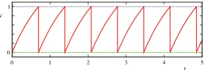
V

Fig. 1. Voltage trace for an LIF oscillator with constant driveI = 2 withτ =

1, vth=1 andvR=0.

where H is the Heaviside step function. The inclusion of the Heaviside term reflects the fact that oscillations do not occur for I

τ < v

th. Electrophysiologists often classify neuron response in terms of the so-calledf

−

Icurve, which shows the frequency of oscillation as a function of the time independent driveI. For the LIF model this is easily constructed from(5)usingf

=

∆−1_{, showing a} sharp rise inf (from zero) asIincreases through the critical value

v

th

/τ

. A plot of the response of the LIF model to constant driveI is shown inFig. 1. Here one sees that the model does not capture the essential shape of a real action potential. Rather the IF model is deemed to be good at capturing the time of generation of an action potential. Since many models of synaptic (chemical) interaction are based on spike-times, rather than spike shapes, this favours the IF model in large scale simulations of synaptically coupled neurons. The tractability of this single neuron model (linear dynamics between firing events) means that it is particularly suited to analysis at the network level with event based models of chemical synapses. Indeed a theory of phase-locked behaviour for strong coupling has been developed for just this scenario [20]. However, gap junction (linear) coupling between neurons means that the action potential shape is communicated from one neuron to another and so LIF models are (without modification) poor candidates for use in this case.

2.2. Nonlinear IF models

The quadratic IF (QIF) neuron is the simplest generalisation of the LIF model that captures qualitatively the behaviour of thef

−

I curve of a large family of more realistic models [21]. Interestingly, this model was apparently already known to Alan Hodgkin, and used to fit some of his data (and also subsequently analysed by Bruce Knight). Up to shifts and constant factors it is defined by

f

(v)

=

v

2

.

(6)

Unlike the LIF model the QIF does allow a representation of an action potential shape (for I

>

0 the voltage rises sharply to threshold), as shown inFig. 2. ForI

<

0 there are two equilibria (one stable and the other unstable) and forI

>

0 these disappear via a saddle–node bifurcation atI

=

0. In the oscillatory regime (I

>

0) the trajectory (for constant drive) can be integrated for Tn

<

t

<

Tn+1to give

v(

t

)

=

√

Itan



tan−1



v

R

√

I



+

√

I

(

t

−

Tn

)



.

(7)

The period of oscillation is calculated by setting

v(

Tn+1

)

=

v

thwith

v(

Tn

)

=

v

Rgiving

∆

=

√

1

I



tan−1



v

th

√

I



−

tan−1



v

R

√

I



H

(

I

).

In the limit

v

th

→ ∞

and

v

R

→ −∞

we see that∆

=

π/

√

I (and we have blowup of the voltage trajectory in finite time), and the f

−

I curve shows a

√

I dependence, which matches many cortical neurons much better than the LIFf

−

Icurve. For a further discussion of this model we refer the reader to the book by Izhikevich [22].

Fig. 2. Voltage trace for the QIF oscillator with constant driveI=1 withvth=10 andvR= −1.

mV

19.5 20.5

t

21.5 22.5

40

-40

[image:3.595.321.535.62.128.2]

-80

Fig. 3. Sample voltage traces (mV) as a function of time (s) from the linear-exponential IF model (green dashed line) and data (red solid line) from a layer-5 pyramidal cell in response to a noisy current injection (constructed from two summed Ornstein–Uhlenbeck processes, see [16] for further details). (For interpretation of the references to colour in this figure legend, the reader is referred to the web version of this article.)

With the improvement in neuronal modelling by simply chang-ing the shape of the nonlinearity from(3) to(6) this raises the question as to whether more judicious choices can improve things further still. Interestingly Fourcaud–Trocmé et al. [23] have shown that choosingf

(v)

=

exp

(v)

(up to shifts and scaling) can act as an approximation of a more detailed conductance-based spiking model. In fact it has now been shown that real cortical data (from layer-5 pyramidal cells) can be very accurately fitted with the fol-lowing choice [16]:

f

(v)

= −

1

τ

(v

−

v

L

)

+

κ

τ

e(v

−v_κ)/κ

_,

(8)

with

v

th

=

30

.

0

, v

R

= −

71

.

2

, v

L

= −

68

.

5

, τ

=

3

.

3

, v

κ

= −

61

.

5 and

κ

=

4.Fig. 3nicely illustrates the strong fit of the model to real data for a stimulation protocol which is a noisy current injection. Similarly to the QIF model the linear-exponential IF (LEIF) model obtained using(8)has two equilibria (defined byf

(v)

+

I

=

0) which disappear in a saddle–node bifurcation whenI

= −

f

(v

∗

₎

_, where

v

∗is defined byf′

(v

∗

)

=

0. In common with the QIF model it is able to support oscillations with arbitrarily low frequency just beyond the bifurcation point. Both the QIF and LEIF models have only a weak dependence on the choice of threshold value since they both blow up in finite time (in the absence of a threshold).

2.3. Planar IF models

Unfortunately, one dimensional nonlinear IF models, as they stand, are unable to reproduce bursting patterns of activity, which are typically associated with slow calcium dependent processes. One way to incorporate such a slow process is by coupling the voltage dynamics to arecoveryoradaptiveprocess in the following manner:

d

v

dt

=

f

(v)

−

a

+

I

,

1

ω

da

dt

=

βv

−

a

.

(9)

[image:3.595.306.549.164.246.2]

-60 -40 -20 0 20 40

0 50 100 150 200

iv) iii)

-60 -40 -20 0 20 40

0 50 100 150 200

ii)

0 50 100 150 200

i)

-60 -40 -20 0 20 40

-60 -40 -20 0 20 40

0 50 150 200

V

100

V

t t

t t

[image:4.595.317.559.61.194.2]

V V

Fig. 4. Firing patterns in the Izhikevich model withI=10 andvth=30. Voltage traces as a function of time for (i) tonic spiking (α=0.02, β=0.2, vR= −65,k= 8), (ii) tonic spiking (α = 0.02, β = 0.2, vR = −55,k = 4), (iii) bursting (α = 0.02, β = 0.2, vR = −50,k = 2), and (iv) fast spiking (α = 0.1, β = 0.2, vR= −65,k=2).

its sensitivity to the choice of threshold value [26]. It is worth noting that a similar model to that of Izhikevich was independently introduced by Gröbler et al. [27] as a model of a pyramidal cell in hippocampus CA3. The adaptive exponential integrate-and-fire model is obtained using a linear-exponential term forf

(v)

(as in Eq.(8)) [28,29], whilst the quartic model is obtained by choosing f

(v)

=

v

4

₊

₂

_ωv

_{[30]. Both are able to produce a wide variety} of firing patterns, and the quartic model in particular has a very nice repertoire of responses ranging from tonic spiking to bursting as well supporting phasic responses, rebound, spike frequency adaptation, sub-threshold oscillations and much more, all of which are discussed in detail in [30].

Apart from the LIF model none of the models described above admits to closed form solutions for arbitrary (non-constant) drive. A somewhat overlooked tractable (one dimensional) nonlinear IF model is that of Karbowski and Kopell [31], with a nonlinearity given byf

(v)

= |

v

|

, which we shall call the absolute IF model (AIF). Because of the choice of a PWL form of the nonlinearity the AIF model can be explicitly analysed. Moreover, it is also capable of generating behaviour consistent with that of a fast-spiking interneuron [32]. The generalisation of the model to allow for bursting behaviour is easily achieved by extending it to the form of (9). A minimal AIF model with adaptation is obtained forf

(v)

= |

v

|

and

β

=

0. For sufficiently smallkthe model fires tonically and for larger values ofkthe model can also fire in a burst mode. The mechanism for this behavior in the AIF model (and indeed all planar models discussed here) is most easily understood in reference to the geometry of the phase-plane. We illustrate, inFig. 5, the phase plane for the AIF model, and refer the reader to [32] for a more detailed discussion and analysis of this model. The analysis of how parameter space partitions into tonic, 1-spike per burst, 2-spike per burst, etc. firing patterns is an open mathematical (classification) challenge. It is worth noting that all the planar models considered here have much in common and can generate a very similar repertoire of firing behaviours, though the AIF model does not have trajectories that blow up in finite time (in the absence of a threshold).

3. Bifurcations of the periodically forced LIF neuron

Because all IF models include a threshold process spikes can be created or annihilated as a voltage trajectory tangentially

Fig. 5. Top left: Tonic firing in the AIF model with spike adaptation. Hereω=1/3 andk = 0.75ω. Top right: Burst firing in the AIF model with spike adaptation. Hereω = 1/75 andk = 2ω. Bottom left: A periodic orbit in the(v,a)plane corresponding to the tonic spiking trajectory shown above (green curve). Also shown is the voltage nullcline (red lines) as well as the value of the reset (blue dashed line). Bottom right: Burst firing in the AIF model with spike adaptation. Here

ω=1/75, andk=2ω. Other parameters arevR=0.2, vth=1 andI=0.1. (For interpretation of the references to colour in this figure legend, the reader is referred to the web version of this article.)

intersects the threshold. This is naturally the case when a time-varying current injection (such as a periodically time-varying synaptic current) is considered (and not just a constant drive). Thus it becomes important not only to assess the stability of spike trains to perturbations that leave the number of spikes unchanged (though do modify firing times), but to address any instabilities that may arise via nonsmooth grazing bifurcations. To show how this can be done we present an analysis of the periodically forced LIF model, though stress that the ideas we present here carry over to more complicated IF models such as those reviewed in Section2.

The phenomenon of mode-locking is well documented in the literature on the periodic forcing of nonlinear oscillators. It is most commonly studied in the context of the standard circle map (see for example [33]). This map is known to support regions of parameter space where the rotation number (average rotation per map iterate) takes the valuep

/

q, wherep

,

q

∈

_Z+_{. These regions} are referred to asp

:

qArnol’d tongues. In a neural context mode-locked solutions are simply identically recurring firing patterns for which a neuron firespspikes for everyqcycles of forcing. With an increase of the coupling amplitude from zero, Arnol’d tongues in the standard circle map typically open as a wedge, centered at points in parameter space where the natural frequency of the oscillator is rational. In between tongues, quasi-periodic behaviour emanating from irrational points on the amplitude/frequency axis, is observed. The technique for calculating such tongues in IF models was first developed by Keener et al. [34] and later expanded upon in [35,36].

Consider a LIF neuron with threshold at

v

th

=

1 and reset level

v

R

=

0 being driven by a∆periodic signalI

(

t

)

=

I

(

t

+

∆

)

. An implicit map of the firing times may be obtained by integrating between reset and threshold according to Eq.(4). Introducing the function

G

(

t

)

=



0

−∞

es/τI

(

t

+

s

)

ds

,

G

(

t

)

=

G

(

t

+

∆

),

(10)

gives

eTn+1/τ

_[

_G

(

_T

n+1

)

−

1

] =

eTn/τG

(

Tn

).

(11)

Defining

F

(

t

)

=

et/τ

[

G

(

t

)

−

1

]

,

(12)

we obtain an implicit map of the firing times in the form

[image:4.595.49.289.64.248.2]

A 1:1 mode-locked solution is defined byTn

=

(

n

+

φ)

∆, with

φ

∈ [

0

,

1

)

, giving a fixed point equation

G

(φ

∆

)

=

1

1

−

e−_∆/τ

.

(14)

Stability is examined by considering perturbations of the form T_n

→

T_n

+

δ

_n, giving

δ

n+1

=

κ(φ)δ

n

,

κ(φ)

=

e

−_∆/τ I

(φ

∆

)

I

(φ

∆

)

−

1

/τ

.

(15)

Solutions are stable if

|

κ(φ)

|

<

1. The borders of the regions where 1:1 solutions become unstable are defined by

κ(φ)

=

1 (tangent bifurcation) and

κ(φ)

=

−

1 (period doubling bifurcation). However, solutions may also lose stability in a nonsmooth fashion in two possible ways, which we shall refer to as type (a) and type (b). In type (a) there is a tangential intersection of the trajectory with the threshold value such that upon variation of the bifurcation parameter the local maxima of the voltage trajectory passes through threshold from above. This is defined by

v

˙

=

−

v/τ

+

I

=

0, so thatI

(

Tn

)

=

1

/τ

or equivalentlyF′

(

Tn

)

=

0. In type (b) a sub-threshold local maxima increases through threshold leading to the creation of a new firing event at some earlier time than usual. This is defined byF

(

T∗

)

=

F

(

Tn

)

+

eTn/τandF′

(

T∗

)

=

0 withT∗

_<

_T

n+1andTn+1is the solution toF

(

Tn+1

)

=

F

(

Tn

)

+

eTn/τ. As an example consider the choice

I

(

t

)

=

I0

+



+

ϵ

0

≤

t

<

∆

/

2

−

ϵ

∆

/

2

<

t

<

∆

.

(16)

In this case the condition

|

κ(φ)

| =

1 is independent of

φ

, since I

(φ)

=

I0

±

ϵ

. A tangent bifurcation occurs when

κ

=

1:

±

ϵ

= −

I0

+

1

/τ

1

−

e−∆/τ

.

(17)

A nonsmooth bifurcation of type (b) is defined by the two equations

τ(

I

+

ϵ)(

1

−

e−∆(1/2−φ)/τ

)

=

1 (18)

v

e−φ∆/τ

+

τ(

I

+

ϵ)(

1

−

e−φ∆/τ

)

=

1

,

(19) where 0

< φ <

1

/

2 and

v

=

e−∆/2τ

+

τ(

I

−

ϵ)(

1

−

e−∆/2τ

).

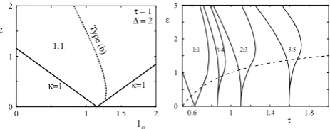
(20) Between them the above two bifurcations define the 1:1 Arnol’d tongue as shown in Fig. 6 (left) (period doubling and type (a) bifurcations are not possible for the parameter values shown). The construction of other tongues with more general values ofp

:

qis carried out in [35,36], and the resultant tongue structure calculated forI

(

t

)

=

I0

+

ϵ

sin 2

π

t is shown inFig. 6(right). Once again the right hand borders of Arnol’d tongues are defined by type (b) nonsmooth bifurcations (and all others by tangent bifurcations of the firing map).

[image:5.595.312.544.62.153.2]

In a pair of recent papers [37,38] it has been shown that spike data from stellate cells in the ventral cochlear nucleus are very well explained by a LIF model with threshold noise, and that Arnol’d tongues are a practical way to understand the way in which single cells in the auditory periphery encode periodic stimuli. Indeed, responses of LIF models to chaotic forcing have also been shown to be largely determined by grazing bifurcations [39]. The techniques described above have also been applied to several variants of the LIF model, including the IF-or-burst model [40], the ‘‘ghostburster’’ model [41] and the resonate-and-fire neuron model [42] as well as to PWL neuron models [43]. Most recently an IF model with a slow T-type calcium current has been studied and been shown to support chaotic behaviour in response to periodic forcing [44]. Interestingly by determining the condition for a grazing bifurcation it was shown that knowledge of unstable periodic orbits (existence

Fig. 6. Left: 1:1 Arnol’d tongue in the LIF model withI(t)a∆-periodic square wave with amplitudeI0±ϵ. Note that a type (b) nonsmooth bifurcation significantly shapes the tongue structure. Hereτ =1 and∆=2. Right:p:qArnol’d tongues in the LIF model withI(t)=I0+ϵsin 2πt. HereI0=2. Below the dashed line the firing map is invertible.

and stability) could be combined with the grazing condition to determine an effective one-dimensional map that captured the essentials of the chaotic behavior. This map is discontinuous and has strong similarities with the universal limit mapping in grazing bifurcations derived in the context of impacting mechanical systems [45]. This latter map was derived for grazing bifurcations that occur in impacting mechanical oscillators and can support period adding cascades with or without chaotic bands.

4. A piecewise linear IF model

The aspect of the LIF model that allows one to perform an analysis such as the one above is obviously its linearity (below threshold). A similar analysis for say the QIF, LEIF or Izhikevich model would be much harder owing to the inherent nonlinear nature of these models. However, the AIF model described in Section 2 is a natural starting point for the development of a more general PWL spiking neuron model that can be explicitly analysed. The use of PWL modelling is already quite common in neuroscience, with the McKean model [3] being a classic example. This may be regarded as a variant of the FitzHugh–Nagumo model [2] that provides a planar model of an excitable cell in which the dynamics is broken into simpler linear pieces. An extension of this approach to develop PWL caricatures of other single neuron models, including the Morris–Lecar model, has recently been pursued by Tonnelier and Gerstner [46] and Coombes [7].

In this section we advocate a new type of PWL IF model, that we shall call the PWL-IF model. It is a generalisation of the AIF model with adaptation that we write in the form of(9)with

f

(v)

=



v

v

≥

0

−

s

v v <

0

.

(21)

For a constant driveIthe model may exhibit a number of different periodic attractors, and in particular we distinguish between those that remain sub-threshold, and those that cross threshold, which we shall term spiking solutions. We make further distinctions between spiking solutions as follows.

Fast spiking orbits:Attracting limit cycles which have

v >

0 along the entire orbit and which have

v(

t∗

₎

₌

_v

that precisely one value oft∗

∈ [

t

,

t

+

∆

] ∀

t, where∆is the period of the limit cycle. Regular (or tonic) spiking orbits:Attracting limit cycles which have

v <

0 for some segment of the orbit and which have

v(

t∗

₎

₌

_v

th at precisely one value oft∗

∈ [

t

,

t

+

∆

] ∀

t, where∆is the period of the limit cycle.

n-Spike bursting orbits:Attracting limit cycles which have

v <

0 for some segment of the orbit and which have

v(

t∗

)

=

v

_that precisely nvalues oft∗

_{∈ [}

_t

_,

_t

₊

_∆

_{] ∀}

_{t, where∆is the period of the limit} cycle.

Fig. 7. Variation of the firing frequency under variation of the driveIfor: Top:

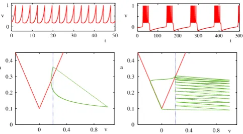
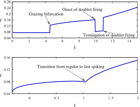
β = 1.2, Bottom:β = 0.9. We can clearly see how the firing rate changes as we move between solution types, and that the firing rate of the model during fast spiking is much more sensitive to changes inIthan in the regular spiking mode.

The fast spiking orbits are so called as they may have arbitrarily fast frequency, whereas the frequency of regular spiking orbits must be finite. With increasingIthe model can make a transition from regular to fast spiking. Contrary to the case for smooth systems, periodic orbits in discontinuous systems need not enclose a fixed point. In fact, the reset mechanism of the PWL-IF model allows for periodic orbits of (9) in the absence of any fixed points. For

β <

1, thef

−

I curve (regular spiking) reaches a maximum value before a bifurcation to fast spiking occurs. The switch between the two modes for

β >

1 may have a further signature of doublet (2-spike burst) firing (which we shall consider in more detail below), and leads to a discontinuousf

−

Icurve.Fig. 7

depicts thef

−

Icurve for differing values of

β

under variation of I. We can clearly see the transitions between the different oscillatory regimes, particularly for

β

=

1

.

2, where we observe discontinuities in the frequency response at a grazing bifurcation, and at the onset and termination of doublet firing.

In order to characterise where in parameter space different types of solution exist, it is useful to consider the different types of bifurcation that can occur. The

v

-nullcline has a characteristic ‘V’ shape, whilst thea-nullcline is a straight line with slope

β

. By inspection, we see that there may exist one, two or no fixed points of(9)withfdefined as in(21). There is a slight subtlety, in that the nullclines may intercept where

v > v

th, generating avirtualfixed point. From here on we refer to the branch of the

v

-nullcline with

v <

0

(v >

0

)

as the left (right)

v

-branch. Since the system is PWL we may easily construct the eigenvalues of fixed points, where they exist, as

2

λ

±

=



1

−

ω

±



(

1

−

ω)

2

₋

₄

ω(β

₋

₁

),

v >

₀

,

−

s

−

ω

±



(

s

+

ω)

2

₋

₄

ω(β

₊

_s

), v <

₀

.

(22)

Thus fixed points on the left

v

-branch are always stable, and the stability of fixed points on the right

v

-branch depends on the sign of 1

−

ω

. The exact nature of the fixed points is determined by the sign of the expression under the square root. Since

β

must be less than 1 to have two fixed points, the fixed point on the right

v

-branch is a saddle.

The sub-threshold dynamics are described by a continuous but non-differentiable system, so that the Jacobian matrix (around a fixed point) at the border separating linear subsystems is not defined. We shall call this border theswitching manifold, as crossing it causes a discontinuous change in the Jacobian. Nonsmooth bifurcations can occur as fixed points or limit cycles touch the

switching manifold under parameter variation. Importantly, the presence of a firing threshold in IF systems means that other nonsmooth bifurcations, and in particular grazing bifurcations as discussed in Section3, can arise.

The PWL-IF can generate periodic behaviour via a Hopf bifurca-tion (HB) of a fixed point on the right

v

-branch when

ω

=

1 (with

β >

1) or through a discontinuous Hopf-like (dHB, black line in

Fig. 8) bifurcation atI

=

0 (with

ω <

1). We describe the sec-ond of these as being discontinuous since the Jacobian around the fixed point changes discontinuously. The emergent sub-threshold limit cycle crosses through the switching manifold

v

=

0. Interest-ingly, with a variation inI, the frequency of the limit cycle does not change (and see [8] for a proof of this), whilst the amplitude grows linearly withI. As the limit cycle grows it can tangentially touch the firing threshold, causing a grazing bifurcation, whereupon sub-threshold oscillations are replaced by regular spiking solutions. In

Fig. 8we may observe both the dHB (black) and the grazing bifur-cation (blue) in

(

I

, β)

parameter space.

Bistability can arise between a stable fixed point on the left

v

-branch and a fast spiking orbit when

β >

1 andI

<

0. In this parameter regime, there exists a saddle node on the right

v

-branch, which is key in delineating the basins of attraction of the two attractors. The basin of attraction of the stable fixed point is the set of initial data such that trajectories reach threshold and are subsequently reset to the right of the separatrix of the saddle on the right

v

-branch. A homoclinic bifurcation (HC), indicated by the blue curve inFig. 8, will occur when the spiking limit cycle collides with the saddle, resulting in a homoclinic orbit from the saddle at the bifurcation point. Another form of bistability is also possible in this parameter regime, namely when a regular spiking limit cycle encloses the stable fixed point. The basin of attraction of this limit cycle is the set of points such that trajectories reach threshold and are reset to the right of the separatrix of the saddle (which is also enclosed by the stable spiking orbit). Numerical studies suggest that the regular spiking orbit is lost as the basin of attraction of the stable fixed point grows and touches the orbit, and as such we shall call this an orbit crisis. As with the HC bifurcation, after this point all trajectories will tend towards the stable fixed point. A plot of the basins of attraction of the two attractors is shown inFig. 9, whilst a plot of parameter values for which we have an orbit crisis is depicted by the magenta (OC) curve inFig. 8. For

β <

1, we have a discontinuous saddle node bifurcation (dSN, orange line inFig. 8) atI

=

0 where the saddle and stable fixed point come together and annihilate one another. We refer to this as a discontinuous bifurcation owing to the fact that the Jacobian of the system is undefined at the bifurcation point. ForI

>

0 there are no fixed points, and the only attractor is either the regular spiking or fast spiking orbit, dependent on the value of

β

. If

β >

1 then the system only possesses one fixed point, which may be on the left or right

v

-branch dependent on the sign ofI. AsIcrosses 0 from below, there are three scenarios: either

ω >

1, in which case no change of stability occurs and trajectories tend to the fixed point, else

ω <

1 and the fixed point becomes unstable. We either may observe sub-threshold oscillations or spiking oscillations (either bursting or tonic) depending on the other parameter values. Using results from [47] we can say more about the sub- or super-critical nature of these bifurcations, though we do not pursue this here. As

β

decreases through

β

c

=

(v

th

−

I

)/v

ththe fixed point no longer exists and we see spiking solutions only.

[image:6.595.54.284.63.238.2]

[image:7.595.51.267.62.221.2]

Fig. 8. Bifurcation curves showing where solution types exchange stability in the

(I, β)parameter plane. Other parameters areω=0.9,s=0.35, vth=60, vR=20 andk=0.4. The dHB refers to the discontinuous Hopf bifurcation, dSN refers to the discontinuous saddle node bifurcation, GB is the grazing bifurcation between sub-threshold oscillations and regular spiking ones, SP is the bifurcation between the regular and fast spiking solutions, HC is the homoclinic bifurcation occurring when the fast spiking orbit collides with the saddle node, OC is the orbit crisis, marking the loss of the regular spiking solution, OB is the bifurcation marking the onset/termination of bistability between sub-threshold oscillations and spiking ones, DB is the bifurcation marking the end of doublet firing, the onset of which occurs along the SP curve. Regions A, B, C, D correspond to bistable parameter regimes, the solutions of which are depicted inFig. 10. Solution types in the other regimes are marked.

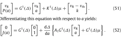
Fig. 9. Basins of attraction for the stable fixed point and limit cycle forω =

0.9, β=0.8,I= −0.2,s=0.35, vth=60, vR=20 andk=0.02. Black denotes the basin of attraction of the stable fixed point whereas white denotes the basin of attraction of the limit cycle. We see that both basins are the union of disconnected sets. The green and yellow circles depict, respectively, the stable fixed point and saddle node whilst the purple dashed lines are the separatrices of the saddle node, given by the eigenvectors of the Jacobian there. The separatrix separates the basin of attraction of the two attractors. The large amplitude limit cycle is lost at the point where it touches the basin of attraction of the stable fixed point. (For interpretation of the references to colour in this figure legend, the reader is referred to the web version of this article.)

where the graze occurs at

v

=

0, the value ofac may be found by integrating backwards from

(v,

a

)

=

(

0

,

I

)

, the point at which

(v,

v)

˙

=

(

0

,

0

)

, a timeT, such that

v(

−

T

)

=

v

_R. The value ofac is then equal toa

(

−

T

)

.T is the flight time (in backwards time) from

v

=

0 to

v

=

v

_Rand may be found numerically. For the case where the graze occurs at

v

=

v

_th, the same method can be used, this time integrating from

(v,

a

)

=

(v

_th

, v

_th

+

I

)

. Interestingly, for bursting orbits, the value ofacmay also be found by finding the curves of inflection of the vector field. These curves separate trajectories that ‘bend’ rightwards, up to the threshold, and those which ‘bend’ leftwards, towards the switching manifold, and are given by the solution to the equation d2a

/

d

v

2

=

0. Substituting

v

=

v

_Rin the resulting equation will giveac. For more discussion about inflection curves, we refer the reader to [8]. In the singular-limit as

ω

→

0, the inflection curve for

v >

0 is precisely the right

v

-branch.

A

B

[image:7.595.312.544.64.221.2]

C

D

Fig. 10. Solution types in the regions indicated inFig. 8. The blue and red solid curves indicate the periodic solutions; all solutions are stable. The orange dashed lines are the branches of thev-nullcline, whilst the sky blue dashed line depicts the

a-nullcline. The green circles in the lower two figures are stable fixed points. (For interpretation of the references to colour in this figure legend, the reader is referred to the web version of this article.)

InFig. 8, we concern ourselves only with non-bursting trajecto-ries. In this case, the graze at

v

=

v

_thresults either in the transition from sub-threshold oscillations to spiking ones, or in the transition from regular spiking orbits to a 2-spike burst. The blue (GB) curve inFig. 8illustrates the first of these cases in

(

I

, β)

parameter space. Where

v

=

0, a graze results in the transition from fast to regu-lar spiking, which may occur after a window of doublet firing. The black curve (SP), inFig. 8corresponds to the transition to regular spiking, either from fast spiking, or from doublet firing, whereas the pink curve (DB) marks the onset/termination of doublet firing. We note that in order to have a graze at

v

thwe require that

β > β

c since we need the

v

-nullcline to be below thea-nullcline for

v

˙

=

0 in this part of the phase-plane.

The number of spikes in a burst is controlled by varying either

ω

, I,

v

R or

v

th. Decreasing any of these parameters will result in bifurcations which decrease the number of spikes in a burst. Where

v

R

<

0, the system is unable to burst as trajectories are always reset to the left of the right

v

-branch and are attracted to the left

v

-branch. We also note that we observe bursts for larger values of

ω

in the case where

β > β

cthan where

β < β

c, and that large values ofImay prohibit bursting, and we observe only fast spiking, so that Iand

β

may be used as control parameters to switch between fast spiking and burst modes.

Owing to the discontinuous nature of the flow at reset, we may observe spiking orbits that enclose all other stable attractors, be they fixed points or sub-threshold oscillations. The emergence of such orbits is controlled by the parameterk. Wherekis too small, trajectories will simply tend towards the attractors whose basin of attraction they are in. However, whenkis large enough, we see the emergence of large amplitude limit cycles. These occur as the flows get ‘interrupted’ as they head towards an attractor in the sub-threshold system. All trajectories starting outside these limit cycles are in the basin of attraction of such orbits.

We illustrate inFig. 10the stable solutions in the various regions of parameter space indicated inFig. 8. The curves inFig. 8 are generated by numerical continuation of solutions obtained from the firing map discussed later in Section6.

5. Periodic orbits and phase response curves

To solve the PWL-IF model it is useful to recast the dynamics in matrix form so that:

˙

X

=



A1X

+

µ

X1

≥

0

,

A2X

+

µ

X1

<

0

,

[image:7.595.42.279.351.477.2]

where

A1

=



1

−

1

ωβ

−

ω



,

A2

=



−

s

−

1

ωβ

−

ω



, µ

=



I 0



,

(24)

withXireferring to theith component ofX(i.e.X1

=

v

andX2

=

a). The solution to the equationX

˙

=

MX

+

µ

can be written using matrix exponentials in the form

X

(

t

)

=

G

(

t

)

X

(

0

)

+

K

(

t

)µ,

(25)

where

G

(

t

)

=

eMt

,

K

(

t

)

=



t

0

G

(

s

)

ds

.

(26)

Explicit solutions forGandK are easily constructed (and see for example [7]). Hereafter, we refer toGi

,

Kias the above expressions with the respective matrixM

=

Ai. To find a fast spiking orbit of period∆(in response to constant forcing) we need only solve

(

X1

(

∆

),

X2

(

∆

))

=

(v

th

,

a0

−

k

)

subject to

(

X1

(

0

),

X2

(

0

))

=

(v

R

,

a0

)

, which gives a pair of simultaneous equations for

(

∆

,

a0

)

as:

v

th

=

G111

(

∆

)v

R

+

G112

(

∆

)

a0

+

K111

(

∆

)

I

,

(27)

a0

=

G1₂₁

(

∆

)v

R

+

K211

(

∆

)

I

+

k 1

−

G1

22

(

∆

)

.

(28)

Bursting orbits may be constructed using similar ideas, though with more book-keeping to keep track of the sub-trajectories (each determined by a linear system) that build the full periodic orbit. For example, for an orbit with ‘times-of-flight’T_i∗

,

i

=

1

, . . . ,

N, (defined by the time spent in a region of phase space before meeting

v

=

0 or

v

=

v

_th) describing a bursting orbit withN

−

2 spikes then we have to solve for the unknowns

(

T∗

1

, . . . ,

T ∗ N

,

a0

)

using a system of equations of the form



0 a1



=

G1

(

T₁∗

)



v

R a0



+

K1

(

T₁∗

)µ,



0 a2



=

G2

(

T₂∗

)



0 a1



+

K2

(

T₂∗

)µ,



v

th

a3



=

G1

(

T₃∗

)



0 a2



+

K1

(

T₃∗

)µ,

...



v

th an



=

G1

(

T_n∗

)



v

R an−1

+

k



+

K1

(

T_n∗

)µ,

(29)

forn

=

4

, . . . ,

Nsubject toa0

=

aN

+

k. The period of the orbit is simply∆

=

N

_i=1T∗

i.

It is common practice in neuroscience to then characterise a neuronal oscillator in terms of its phase response to a perturbation. This gives rise to the notion of a phase response curve (PRC). The PRC quantifies the phase shift of an oscillator due to a small, brief perturbation as a function of the phase of the oscillator when the perturbation occurred. A positive phase response indicates an advancement in the timing of the next oscillation, while negative values indicate a delay. For a detailed discussion of PRCs we refer the reader to [48]. One way to compute them for a given smooth dynamical system is via the Malkin adjoint method. Following [49] we briefly review this approach. Consider a smooth dynamical systemz

˙

=

F

(

z

),

z

∈

_Rn_{, with a∆-periodic solutionZ}

₍

_t

₎

₌

Z

(

t

+

∆

)

and introduce an infinitesimal perturbation1z0to the trajectoryZ

(

t

)

at timet

=

0. This perturbation evolves according to the linearised equation of motion:

d1z

dt

=

DF

(

Z

(

t

))

1z

,

1z

(

0

)

=

1z0

.

(30)

Here DF

(

Z

)

denotes the Jacobian ofF evaluated alongZ. Intro-ducing a time-independent phase shift1

θ

as

θ(

Z

(

t

)

+

1z

(

t

))

−

θ(

Z

(

t

))

, we have to first order in1zthat

1

θ

= ⟨

Q

(

t

),

1z

(

t

)

⟩

,

(31)

where

⟨·

,

·⟩

defines the standard inner product, andQ

= ∇

_Z

θ

is the gradient of

θ

evaluated atZ

(

t

)

. Taking the time-derivative of

(31)gives



dQ

dt

,

1z



= −



Q

,

d1z

dt



= −⟨

DFT

(

Z

)

Q

,

1z

⟩

.

(32)

Since the above equation must hold for arbitrary perturbations, we see that the gradientQ

= ∇

_Z

θ

satisfies the linear equation

dQ

dt

= −

DF

T

₍

_Z

₍

_t

₎₎

_Q

_,

₍₃₃₎

subject to the conditionsQT

(

0

)

F

(

z

(

0

))

=

1

/

∆andQ

(

t

)

=

Q

(

t

+

∆

)

. The first condition simply guarantees that

θ

˙

=

1

/

T (at any point on the periodic orbit), and the second enforces continuity (and periodicity). The (vector) PRC,R, is related toQ according to the simple scalingR

=

Q∆. In general(33)must be solved numerically to obtain the PRC, say, using theadjoint routine in XPP [50]. However, for PWL models DF

(

Z

)

is piecewise constant, and we can obtain a solution in closed form [7]. Moreover it is also possible to extend the Malkin method to treat an IF process [32], which would give rise to a discontinuous PRC (at the spike time). In this latter case the continuity condition is swapped in favour of enforcing the normalisation conditionQT

₍

_t

₎

_F

₍

_z

₍

_t

₎₎

₌

₁

_/

_∆for allt.

For the PWL-IF model we may constructQ in given regions of phase space according to the prescriptionQ

(

t

)

=

J

(

T_i∗

−

t

)

Q

(

T_i∗

)

, where J

=

GT _{(and see [7] for further details). Enforcing the} normalisation condition at the times T∗

i is enough to define a periodic (yet discontinuous) form forQ. For example, for a simple tonic spiking orbit we see that solving (33)and imposing the normalisation condition att

=

0 andt

=

∆gives a system of two linear equations in

(

q1

,

q2

)

, whereqiare the components ofQ as

q1

(

∆

)(v

th

+

I

−

a0

+

k

)

+

q2

(

∆

)ω(βv

th

−

a0

+

k

)

=

1

∆

,

q1

(

0

)(v

r

+

I

−

a0

)

+

q2

(

0

)ω(βv

r

−

a0

)

=

1

∆

.

(34)

Using the further result thatQ

(

0

)

=

ΓQ

(

T

)

whereΓ

=

J1

₍

_∆

₎

_for fast spiking orbits orΓ

=

J1

₍

_T∗

3

)

J2

(

T ∗ 2

)

J1

(

T

∗

1

)

for regular spiking orbits, gives

q2

(

∆

)

=

r1

−

r2Γ11

−

r4Γ21

T

(

r1

(

Γ12r2

+

r4Γ22

)

−

(

r3r2Γ11

+

r3r4Γ21

))

,

q1

(

∆

)

=

1 r1



1

∆

−

r3q2

(

∆

)



,

(35)

where

r1

=

v

th

+

I

−

a0

+

k

,

r2

=

v

R

+

I

−

a0

,

(36)

r3

=

ω(v

th

−

a0

+

k

),

r4

=

ω(v

R

−

a0

).

(37)

Hence for a fast spiking orbit the adjoint is given byQ

(

t

)

=

J

(

∆

−

t

)

Q

(

∆

)

and for a regular spiking orbit the correspondingQ is

Q

(

t

)

=







J1

(

T₁∗

−

t

)

J2

(

T₂∗

)

J1

(

T₃∗

)

Q

(

∆

)

0

≤

t

≤

t1 J2

(

T₂∗

−

t

)

J1

(

T₃∗

)

Q

(

∆

)

t1

≤

t

≤

t2 J1

(

T₃∗

−

t

)

Q

(

∆

)

t2

≤

t

≤

∆

,

(38)

where tj

=

j

i=1T ∗

[image:9.595.52.263.62.220.2]

Fig. 11. Left: Voltage component of the phase response curve for a regular spiking orbit (red, solid). Right: Voltage component of the phase response curve for a 3-spike bursting orbits (red, solid). Parameter values areβ=1.1,s=0.35,k=0.4 andω = 1 for the regular spiking orbit andω = 0.25 for the bursting orbit. Corresponding orbits are shown in dashed blue. (For interpretation of the references to colour in this figure legend, the reader is referred to the web version of this article.)

same way, except that discontinuities are now not isolated to the ends of the periodic orbit, and so we must enforce both the normalisation condition just before and just after each threshold crossing. Typically, when studying neural oscillators, we are primarily concerned with the first (voltage) component ofQ, since perturbations to the system are usually given by changes in the external current, which acts only on the voltage variable. As an example we plot inFig. 11the voltage component ofQfor a regular spiking orbit and a burst containing three spikes. Knowledge of the PRC is fundamental in building network descriptions of weakly coupled oscillators [51], and for PWL models is discussed in more detail in [7].

To study the stability of tonic spiking orbits (and for simplicity we focus here on the case that

v >

0), we rewrite Eq.(23)as

dX

dt

=

MX

+

µ

+

d



n

δ(

t

−

Tn

),

t

≥

0

,

(39)

with

d

=



v

R

−

v

th

k



.

(40)

Integrating Eq.(39)between two successive firing times yields the closed form expression

X−

(

Tn+1

)

=

G

(

∆n

)

[

X−

(

Tn

)

+

d

] +

K

(

∆n

)µ,

(41)

with∆n

=

Tn+1

−

Tn. The superscript onXin Eq.(41)indicates that we evaluateXat the firing eventbeforethe reset, i.e.X−

(

Tn

)

=

lim_ε↘0X

(

Tn

−

ε)

. For later reference, we here also introduce X+

(

Tn

)

=

limε↘0X

(

Tn

+

ε)

and note thatX+

(

Tn

)

=

d

+

X−

(

Tn

)

. A perturbation of the periodic orbits with a period∆leads to perturbed firing times



Tn, for which we make the ansatz



Tn

=

n∆

+

δ

Tn. Similarly, we write the perturbed trajectory as



X

(

t

)

=

s

(

t

)

+

δ

X. Hence, we have from Eq.(41)



X −

₍

Tn+1

)

=

G

(



∆n

)

[



X −

₍



Tn

)

+

d

] +

K

(



∆n

)µ,

(42)

where



∆n

=



T_n+1

−



T_n. Linearising equation(42)then results in

δ

Xn+1

=

eM∆

δ

Xn

−

δ

TneM∆p

+

δ

Tn+1q

,

(43) with

p

=

M

[

s−

(

∆

)

+

d

] +

µ

= ˙

s+

(

∆

),

(44a)

q

=

Ms−

(

∆

)

+

µ

= ˙

s−

(

∆

),

(44b)

where

δ

Xn is defined through



X

(

T_n

)

=

s

(

T_n

)

+

δ

X_n and

˙

s

=

ds

/

dt. At first sight, Eq.(43)appears to be implicit since

δ

Xn+1 is given in terms of the unknown perturbation of the firing time

δ

Tn+1. However, we need to solve Eq. (43)with the constraint that

_

v(



T_n−

)

=

v

th

=

v(

Tn−

)

, so that the first component of

δ

Xn+1vanishes. Defining the row vector

γ

with components

γ

i

=

−[

eM∆

]

_1i

/

[

q

]

₁, we find for the perturbed firing time

δ

Tn+1

=

γ (δ

Xn

−

p

δ

Tn

),

(45)

which immediately leads to

δ

Xn+1

=

(

eM∆

+

q

γ )(δ

Xn

−

p

δ

Tn

).

(46) Hence, the perturbations ofX at the

(

n

+

1

)

th firing time are uniquely determined by the perturbations at thenth firing event. From Eq.(45), we see that

δ

Xn

−

p

δ

Tn

=

(

eM∆

−

Md

γ )(δ

Xn−1

−

p

δ

Tn−1

).

(47) Without loss of generality, we set

δ

T0

=

0 att

=

0, which is equivalent to saying that there is some perturbation of the periodic orbit att

=

0. Then, Eqs.(45)and(46)yield

δ

T1

=

γ δ

X0 and

δ

X1

=

(

eM∆

+

q

γ )δ

X0, so that we find from Eqs.(46)and(47)

δ

Xn+1

=

(

eM∆

+

q

γ )(

eM∆

−

Md

γ )

n

δ

X0

.

(48) Hence, the perturbations grow without bound if there is at least one eigenvalue ofB

=

(

eM∆

₋

_Md

_{γ )}

_{with modulus larger than one.} Conversely, if all eigenvalues ofBhave moduli smaller than one, then any initial perturbation decays towards zero. However, our analysis indicates thatBalways possesses exactly one eigenvalue equal to 1, so thatBn_{converges against a constant matrixBfor large} ninstead of decaying if all other eigenvalues have moduli smaller than one. The stability of the period one orbit is then determined by the product

(

eM∆

+

q

γ )

B. For the parameter values where fast spiking orbits exist (e.g.I

=

4

.

0

,

k

=

0

.

4

, v

th

=

60

, v

R

=

8

.

1

, β

=

0

.

5

,

s

=

0

.

35

, ω

=

0

.

08) we find that this product equals zero, so that the orbit is asymptotically stable. The above argument relies on the numerical evaluation of the matrices and eigenvalues. A more detailed study on the structure ofBwill be reported elsewhere.

Next we show how to determine single neuron behaviour (existence and stability) via an alternative approach based on the construction of a discontinuous one-dimensional return map.

6. Firing map

Due to the nature of the nonsmooth dynamics of the system at reset, it is useful to consider a map of the adaptation variable at successive firing times. This will collapse the dynamics of the full system to a one-dimensional return map. This has previously been considered by Touboul and Brette [52] for a broad class of planar nonlinear IF models. Here, we focus on the construction of such a map for the PWL-IF model. We consider a set, called the Poincaré section,Σ

= {

(v,

a

)

|

v

= ¯

v

∈

_R

}

which is transverse to the flow for all

(

v,

¯

a

)

∈

Σ. The value of

v

¯

above is arbitrary, so that our section may be placed anywhere in the phase plane. The first return map is a function which gives, for each valuea0

∈

R, the value

ofaat the next intersection withΣ, of a trajectory starting from

(

v,

¯

a0

)

. The second return map gives the second intersection of such a trajectory withΣand so forth. We refer to the firing map as the first return map with

v

¯

=

v

_R. We note that trajectories will not intersect

v

Rupon reaching threshold, but are reset discontinuously to it, and thus we may consider intersection of the trajectory with