(will be inserted by the editor)
A New Model and a Hyper-heuristic Approach for Two-dimensional
Shelf Space Allocation
Ruibin Bai1, Tom van Woensel2, Graham Kendall3 and Edmund K. Burke4
1 Department of Computer Science, University of Nottingham Ningbo China, 199 Taikang East Road, Ningbo, China, 315100,
Tel. +86-574-88180278, Fax +86-574-88180125. e-mail:[email protected].
2 School of Industrial Engineering, Technische Universiteit Eindhoven, Den Dolech 2, Pav. F05, Eindhoven NL 5600 MB, The
Netherlands. e-mail:[email protected].
3 School of Computer Science, University of Nottingham, Nottingham, UK and Semenyih, Malaysia.
e-mail:[email protected]
4 Department of Computing Science and Mathematics, University of Stirling, Cottrell Building, Stirling, FK9 4LA, UK. e-mail:
Received: September 2011 / Revised version:
Abstract In this paper, we propose a two-dimensional shelf space allocation model. The second dimension stems from the height of the shelf. This results in an integer nonlinear programming model with a complex
form of objective function. We propose a multiple neighborhood approach which is a hybridization of a
simulated annealing algorithm with a hyper-heuristic learning mechanism. Experiments based on empirical
data from both real-world and artificial instances show that the shelf space utilization and the resulting
sales can be greatly improved when compared with a gradient method. Sensitivity analysis on the input
parameters and the shelf space show the benefits of the proposed algorithm both in sales and in robustness.
1. Motivation
Retailers aim to maximize availability of the goods in their product line at a minimum cost to operations. In
the stores, these goals have to be realized on the shelves, where any product meets the customer. Shelf spaces
are expensive resources for many retail stores and supermarkets. Space planning and shelf operation is thus
a major area that can significantly improve a retailer’s financial performance and customer satisfaction.
One of the responsibilities of marketing is designing an attractive presentation on the shelves in order
to attract customers. The amount of shelf space allocated to a product is thus primarily a consequence
of marketing decisions: i.e. the merchandizing category to which the product is assigned and the allocated
number of facings (the number of slots on the front of a retail shelf). Planograms (Bai and Kendall, 2005)
represent plans of how retail products will be laid out on the shelves, and show retailers where and how each
Stock Keeping Unit (SKU) should be displayed. SKUs are used to uniquely identify a specific product or
goods in location and its characteristics. It is the smallest management unit in a retail store. Planograms
determine the available shelf space for the operations. From both an operations and a marketing point of
view, it is thus important to produce high-quality planograms.
A planogram contains important information for the execution of the operations. In general, when
con-structing planograms the retailer decides on the assortment composition (which items are in the assortment?),
the location of the item in the stores (where are the aisles, section, and shelf locations?) and the amount of
space allocated to each item (how many facings and consumer units?). In an empirical study by Van Woensel
et al. (2006), it was observed that planogram integrity is a serious issue for retailers. Planogram integrity is
the degree to which the planograms are followed in practice. The empirical evidence clearly demonstrated
that the majority of differences are mainly due to facing differences. In second and third place of
impor-tance, it was found that assortment and location differences are important. A major consequence of a lack
of planogram integrity is the loss of a substantial level of efficiency both in terms of the marketing strategy
as well as in the operational executions.
An important underlying driver for these planogram integrity problems, could be related back to the
inability of the planogram tools to cope with real-life situations. The store managers tried to remedy this
by taking into account a greater number of factors and changing the proposed planograms. In general, the
motivation relates back to the issue that planograms are mainly built based on marketing decision rules (e.g.
the number of facings per product category) and are often one-dimensional (i.e. do not take into account
the depth nor height of the shelves). This paper takes a significant step towards more efficient planograming
effects of shelf space on the demand. Moreover, we proposed an efficient hyper-heuristic method for tackling
this two-dimensional plangram problem.
The paper makes the following contributions:
– Most of the shelf space allocation models discussed in the literature treat shelf space one-dimensionally, quantified either in volume or in shelf length. That is, the capacity of shelf is usually quantified as a single
real value (see e.g. (Corstjens and Doyle, 1981; Dreze et al., 1994; Urban, 1998; Yang, 2001; Hwang et al.,
2005; Bai and Kendall, 2008)). These models are mainly useful if all the shelves and items concerned
have similar height dimensions and it is impossible to improve the space utilization by manipulating
items across shelves. These models are also useful when items cannot be stacked for various reasons (for
example wine and milk bottles). Our paper presents a 2-dimensional approach taking into account not
only shelf length but also shelf height. In addition, the paper proposes a hyper-heuristic based approach
which can potentially handle large-sized problem instances.
– Today, many items can be stacked together in order to make full use of the shelf space with regard to the height dimension, but this is not explicitly considered in current planogram optimization tools. Of
course, in practice shelf operators can still stack items on top of the facings allocated according to a
one-dimensional model. However, this usually leads to decreased space utilization and productivity. We
show, via a rigorous scale of experiments, that explicitly taking into account the height dimension will
improve the space utilization.
The paper is structured as follows: Section 2 discusses related work. Section 3 formulates our model of the
shelf space allocation. Methodologies that are used to optimize the problem model are presented in Section
4. Numerical examples are presented in Section 6 along with sensitivity analysis on parameter estimation
errors and Section 7 concludes the paper.
2. Related Work
The study of shelf space allocation dates back to the 1960’s with some empirical experiments being carried
out to study the influence of shelf space operations. For example, Kotzan and Evanson (1969) made empirical
studies for three products from eight chain stores and found that a significant relationship existed between
shelf facings and sales. Cox (1970) carried out similar experiments for products from two brands of two
categories, salt and coffee cream. He reported a very weak relationship between shelf facings and sales.
Space elasticity has been widely used to measure the responsiveness of the sales with regards to the
to relative change in shelf space” and reported an average value of 0.212. However, this is just an average
value: the actual value of the space elasticity can be very different, depending on the products, stores and
in-store layout (Curhan, 1973). Cross-product effects were also investigated in (Dreze et al., 1994) where space
manipulations were made to enhance complementary shopping by placing complementary products together.
The results showed that complementary merchandizing resulted a positive boost in sales (over 5%) on the
tested products (toothbrush, toothpaste and laundry care). It was also found that, compared with shelf
facings, location had a larger impact as long as a minimum number of shelf facings (to avoid out-of-stocks)
was maintained. Shelves at the eyesight level are more favorable than shelves located at the top or bottom of
the shelf fixtures. Quantitative models have been proposed to describe the relationship between shelf space
and sales. Corstjens and Doyle (1981) firstly formulated their model in a non-linear multiplicative way and
incorporated cross elasticities, a set of problem parameters that reflect the interrelationships between the
different products under consideration. The inventory and handling cost effects were also considered. Two
parameter estimation approaches were also compared and discussed. Zufryden (1986) proposed a dynamic
programming model for the shelf space allocation problem, which also took into account some non-space
factors such as price, advertising, promotion, store characteristics, etc. However, the approach may only be
suitable for small sized problems and becomes computationally expensive for larger problem instances.
Recognizing that shelf space allocation is also closely related with other retailing problems, some
in-tegrated models have also been proposed. For example, Borin et al.’s model (Borin et al., 1994) could
simultaneously provide a solution for both product assortment and shelf space allocation. A simulated
an-nealing algorithm was used to optimize the proposed model. Urban (1998) integrated product assortment
and inventory control with a traditional shelf space allocation model. A genetic algorithm was proposed to
solve the problem. However, these models usually involve a large number of parameters. Obtaining a reliable
estimation of these parameters is generally challenging and time-consuming. Therefore, it is difficult to put
these models into a real application. A simplified linear model was proposed in (Yang, 2001), which
consid-ered the location effect of shelves on sales. The model, in fact, is a varied type of bounded multi-knapsack
problem, which is generally difficult to solve. The authors designed several greedy heuristics to optimize the
problem model.
However, these simple heuristics will only return a sub-optimal solution in many cases due to their inability
to escape from local optimality. To solve the weakness of these simple heuristics, Lim et al. (2004) proposed
several approaches, including a network flow procedure, tabu search and a modified squeaky-wheel algorithm.
Experimental results, over several problem instances, showed that the modified squeaky-wheel algorithm is
shelf space allocation model was proposed in (Hwang et al., 2005) which considers both the inventory and
location influence on the demand. Both a gradient-based procedure and a genetic algorithm were used to solve
the problem and experimental results on several small numerical instances showed that the genetic algorithm
is able to obtain superior results. Bai and Kendall (2008) proposed an integrated inventory and shelf space
allocation model specifically to handle fresh produce. A modified generalized reduced gradient approach was
used to search for good quality solutions. Murray et al. (2010) and Hwang et al. (2009) have presented shelf
space allocation models related to the one presented in our paper. Specifically, Hwang et al. (2009) looked
into a simultaneous shelf space design and allocation problem. A mathematical model was developed and two
solution procedures were proposed based on a genetic algorithm (Goldberg, 1989; Sastry et al., 2005). This
was applied to some very small test instances of four products. Murray et al. (2010) developed a model that
jointly optimizes a retailer’s decisions for product prices, display facing areas, display orientations and
shelf-space locations in a product category. This comprehensive model is solved by branch-and-bound procedures
on some small test instances. Our paper is distinct by the use of hyper-heuristics and the ability to solve
larger, more realistic sized instances.
Hyper-heuristics (Burke et al., 2003a; Ross, 2005) have recently received increasing attention partly
because one of their motivating goals is to establish a higher level of generality across different problem
solving scenarios. A hyper-heuristic searches across a space of heuristics rather than the more usual heuristic
approach of dealing with the solution space directly. Hyper-heuristics have successfully been applied to
several difficult search problems, including timetabling and rostering (Burke et al., 2003b; Bai et al., 2012;
Burke et al., 2006, 2007), scheduling (Hart et al., 1998), and packing and layout optimization (Bai et al.,
2008; Dowsland et al., 2007).
3. Model Development
In a similar way to that presented in (Yang, 2001), it is assumed that retailers can prevent going out-of-stock
by improving their supply chain. Space allocation is carried out within a given category (space allocation
between different categories is usually a strategic problem rather than a quantitative one). Shelves are in
multi-level with each level having a different impact factor. The problem can be formulated as follows: we
are given a number of shelvesm with each shelf j having a demand impact factorγj (γj ≥1) and we are
also given a number of nSKUs. The least popular shelves (i.e. either the bottom or the top shelves) have
an impact factor of 1 and shelves that are close to “eye-level” haveγi values greater than 1. An SKU can
allocate an appropriate number of facings to each SKUisuch that the total sales of the SKUs are maximized.
[image:6.595.153.463.162.434.2]The notations used in the model are defined in Table 1.
Table 1.List of variables used in the analysis
Description
Lj Length of shelf j
Hj Height of shelfj
li Length of SKUi
hi Height of SKU i
πij Stack coefficient of item ion shelfj, andπij =⌊ Hj
hi⌋
Fi Demand function of item iover time
Mi Sales realized on itemi
αi Scale parameter for demand function of itemi
βi Space elasticity for item i
βik Cross elasticity of item kon itemiandβik is asymmetric.
γj Location impact factor of shelf j
pi Unit selling price of itemi
smin
i Minimum number of facings for itemi
smax
i Maximum number of facings for itemi
xij length facing of shelfj allocated to itemi
xi Total shelf length facings allocated to itemi, i.e. xi= m
∑
j=1 xij
si Total facings allocated to itemi
yij yij= 1, if item iis placed on shelfj
yij= 0, if item iis not placed on shelfj
zi Shelf ID on which product iis displayed
For simplicity, we define length facing as the number of facings that are allocated to an item along
the shelf length and stack coefficient as the maximum number of facings that can be allocated in height.
Therefore, the total number of facings of an item is the product of length facings and the stack coefficient.
We use the same deterministic demand function proposed by (Hwang et al., 2005). In their paper, they
formulated the demand function as a multiplicative form of direct space effect, cross space effect and location
effect:
Fi=αi×sβii×[ n
∏
k̸=i
sβik
k ]×Υi (1)
where si is the total number of facings allocated to item i. For a stacking coefficient value πij, si can be
calculated as
si= m
∑
j=1
andΥi the average location effect obtained as
Υi=
∑m
j=1xijπijγj si
(3)
The model can then be formulated as follows
max
n
∑
i=1 Mi =
n
∑
i=1
piFi (4)
subject to:
n
∑
i=1
lixij ≤Lj,∀j (5)
yij ≤πij,∀i, j (6)
smini ≤si≤smaxi ,∀i (7)
xij ∈ {0} ∪Z+,∀i, j (8)
yij ∈ {0,1},∀i, j (9)
yij ≤xij,∀i, j (10)
yij×Lj/li ≥xij,∀i, j (11)
m
∑
j=1
yij = 1,∀i (12)
Constraints (5) and (6) make sure that the items allocated to each shelf do not exceed the capacity of
the shelf (both in length and height). Constraint (7) defines the minimum and maximum facings which can
be allocated to each item. Constraints (8), (9), (10) and (11) define the integrality of decision variablesxij
andyij and their relationships. Constraint (12) is a cluster constraint which ensures that the same type of
items have to be displayed together on one shelf. The cluster constraint is not considered in previous models,
which means that the same type of items can be displayed on several different shelves. In practice, retailers
usually want to keep the same type of items in the same place to present a large attractive block. Therefore,
this constraint is included in our model.
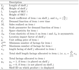
To illustrate the necessity to use a 2D model, we now consider one of the 1D numerical examples presented
in (Hwang et al., 2005). The example is drawn from the Dataset1 with 4 “mixed” items (i.e. including both
substitutive and complementary items) and 4 shelves. For completeness, the details of the problem instance
Table 2.A numerical example taken from (Hwang et al., 2005)
βik
itemi pi li smini smaxi αi 1 2 3 4
1 5.89 1 1 6 62.26 0.500 0.011 -0.014 -0.010
2 4.37 1 1 6 70.11 0.010 0.250 -0.009 0.014
3 4.91 1 1 6 66.92 -0.005 -0.006 0.400 -0.011
4 6.14 1 1 6 61.22 -0.008 0.009 -0.015 0.340
Shelf data:m= 4,Lj ={3,3,3,3},γj ={1.3,1.2,1.1,1.0}
The optimal solution (obtained by an exhaustive search procedure) for this 1D problem instance is
displayed in Fig. 1 (a). As can be seen, this example assumes that both shelves and items have unit height
sizes. In reality, however, shelves are often in different heights (ranging from 100mm to 1000mm based on
our own data) and items can be stacked if the shelf space and other conditions allow it. Now suppose that
the fourth shelf is two units in height instead of one. If the 1D planogram solution is still used, one would
probably come up with a solution by stacking three more of item 2 onto the fourth shelf (corresponding to
Fig. 1 (b)). This solution gives an objective value of 2492.55. However, the true optimal solution is 2616.29
which is shown in Fig. 1 (c). The retailer could potentially lose 123.74 worth of sales in this case. This simple
example shows that using a 1D planogram model can lead to considerable losses. It should be noted that, in
this example, we only slightly changed the original data instance (one shelf only). In practice, both shelves
and items may be of a different height, which justifies the necessity of using a two-dimensional planogram
model, although item heights are not critical: (1) if the shelves are of the same height, the problems with
items of different heights could be easily transformed into a one-dimensional problem; (2) even if the items are
of the same height, the problems with shelves of different heights can be transformed into a one-dimensional
problem.
4. Solution Approaches
The problem presented in (4) subject to (5)-(12) is an integer nonlinear programming model with a complex
form of objective function. The decision variables arexij. Due to the cluster constraint (12), each item can
only be displayed on one shelf. Therefore, the solution can be represented by the following two vectors: let
zi be the shelf ID on which itemi is displayed. Letxi be the shelf length facings that are allocated to item
i. This reduces the number of decision variables to 2n. Given this, the problem is still very difficult to solve
in a closed form. A complete search algorithm is also prohibitive even for a medium sized problem. We
Fig. 1.A comparison of a 1D planogram with a 2D planogram (a) Optimal solution for the 1D planogram. (b) the 1D planogram when shelf height changed. (c) Optimal solution of the 2D planogram
approaches have been widely used to solve several shelf space allocation or related problems (Borin et al.,
1994; Urban, 1998; Yang, 2001; Lim et al., 2004; Hwang et al., 2005; Bai et al., 2008).
4.1 A gradient approach
Because of the limited shelf space resources, items compete against each other for space. A gradient approach
iteratively allocates shelf space to the items that can produce the largest reward per unit space in terms
of the objective value (in this case, sales). However, due to the nonlinearity of the objective function, the
ratio of sales to the allocated space varies with different shelf facing valuessi. The partial derivative of the
objective function with regard to decision variables xuv (u=1,..n, v=1,...,m) is quite complex and can be
presented as follows:
∂
n
∑
i=1 Mi
∂xuv
=∑
i̸=u
[piαiβiuπuvsβii−1s βiu−1 u
∏
k̸=i,u
sβik k
m
∑
j=1
(xijπijγj)] +
puαuπuvsβuu−2
∏
k̸=u
sβuk
k [(βu−1) m
∑
j=1
(xujπujrj) +suγv] (13)
Due to the minimum facing constraint (7), most constructive heuristics for shelf space allocation problems
space to each item so that the minimum facing requirements are satisfied. In the second phase, the algorithm
then repeatedly allocates the remaining space to the most preferable items according to some criteria. For
example, the partial derivative function (13) would be a good candidate for this purpose. We can simply
repeatedly increase the value ofxuv that gives the largest partial derivative value according to function (13),
assuming there is still sufficient space available on shelfv. If this is not the case, the second largest partial
derivative value is chosen, and so on. However, there is a problem. The existence of the cluster constraint
(12) means that each item can only be displayed on one of the shelves. Therefore, once the first facing of an
item is allocated to a given shelf, the remaining facings of this item have to be on the same shelf. This means
that the first phase of the procedure is paramount in terms of the accommodating shelf for each item. If
function (13) is adopted directly in the first phase of the algorithm, the algorithm tends to allocate the first
facing of most of items to the most attractive shelves and leaves some of the less attractive shelves empty.
To solve this problem, the gradient algorithm used in this paper selects shelves based on the following rules,
instead of function (13). At each iteration, the shelf with largest residual length is selected, with ties broken
by favoring larger shelf heights and then the location impact factor.
The algorithm can be described as follows:
S1. Initial Phase
S1.1 Select a shelf v with the largest residual capacity, with ties broken by favoring larger shelf height
and then the larger location coefficient.
S1.2 For each itemuthat has not been initialized, setsu=sumin,xu=⌈su/πuv⌉,su=xu×πuv,zu=v.
S1.3 Calculate the partial derivative according to function (13), select the item that has the largest partial
derivative value and that can be accommodated by the shelfv. Label this item to be initialized.
S1.4 If all items are initialized, go to S2, otherwise, go to S1.1.
S2. Iterative Phase
S2.1 For each item and its accommodating shelf, update the corresponding derivative value according to
function (13). Sort the items according to the descending order of their derivative values.
S2.2 Select the first item u in the list, denote v be the shelf on which u is placed, set xu = xu+ 1,
su=su+πuv. If this results in an infeasible solution, setxu=xu−1,su=su−πuv and exclude this item
from further consideration.
4.2 A Multi-neighborhood Approach
Metaheuristics (Glover and Kochenberger, 2003) have been widely used to tackle highly constrained
opti-mization problems from various fields. Multiple neighborhood search approaches have recently emerged as
a popular meta-heuristic technique because of their ability to handle difficult constraints and obtain high
quality solutions. Utilizing multiple neighborhoods could increase the accessibility of the search space and
also improve the efficiency of the local search.
In this paper, a hybrid multiple neighborhood approach is proposed to solve this two-dimensional shelf
space allocation problem. The multiple neighborhood approach utilizes a collection of neighborhoods in
hybridization with a simulated annealing algorithm and a hyper-heuristic (Burke et al., 2003a; Ross, 2005)
learning mechanism. This approach has shown considerable generality and competitiveness across large
num-ber of datasets of two very different combinatorial optimisation problems (bin packing and university course
timetabling) (Bai et al., 2012). The increased generality is achieved by preventing hyper-heuristic from
us-ing problem-dependent information. Fig. 2 gives a pseudo-code of this approach. Based on a given initial
solution and a set of neighborhoods, this hyper-heuristic approach intelligently changes the neighborhood
preferences during the search and the simulated annealing is used to determine whether a given
neighbor-hood move suggested by the hyper-heuristic is accepted or rejected. More specifically, each neighborneighbor-hood is
associated with a weightwi to represent its preference in comparison to the other neighborhoods. At each
iteration, a neighborhood is stochastically ranked by the probabilitypi =wi/
∑n
i=1wi. Initially, weights are
set to a predefined common minimum wmin and then updated periodically (defined by a learning period,
or LP). Performance of each neighborhood in a given learning period is monitored and measured by two
criteria, namely acceptance ratio and percentage of new solutions being generated. During normal
“anneal-ing” phase, the weight wi is set to the acceptance ratio of each heuristic in the previous period and then
stays unchanged during the learning period. If, however, at the end of the period the average acceptance
ratio among all neighborhoods falls below a threshold, a “reheating” strategy is triggered to diversify the
search and neighborhoods that are more likely to generate new solutions are favoured. Interested readers
could refer to (Bai et al., 2012) for more discussions about this approach and its relationship with some of
other metaheuristics, for example, iterated local search, variable neighbourhood search and adaptive large
neighborhood search approaches.
N1 Swap:This neighborhood includes all the neighboring solutions that can be generated by swapping one shelf length facing of two itemsi,kthat are sharing the same shelf in the current solution. i.e.xi =xi+ 1,
xk=xk−1.
N2 Shift: This neighborhood aims to improve the current solution by changing an item’s current accom-modating shelf. The neighborhood consists of all the solutions that can be generated by moving all the
facings of an item from its current shelf to a different shelf.
N3 Interchange:This neighborhood enables the algorithm to interchange two items’ (i,k) accommodating shelves if they are different (i.e.zi ↔zk). This neighborhood is different from N1 in that it operates on
the facings of items from two different shelves while N1 operates on the items’ facings on the same shelf.
N4 Add Facing: This neighborhood consists of all the neighboring solutions that can be generated by increasing the length facingxi of itemiby one.
N5 Delete Facing:This neighborhood function deletes a length facing of a randomly selected item.
4.2.2 Constraint handling Since not all of the above neighborhood moves produce feasible solutions, a
mechanism has to be used to ensure that the algorithm searches within feasible regions of the search space.
In this paper, the following method is used. For neighborhoods N1, N4 and N5 that involve adding/deleting
facings to/from a single shelf, if a neighborhood move leads to an infeasible solution, the move is rejected
and the search goes back to the previous point. For neighborhoods N2 and N3, if the solution is not feasible
because of violations of shelf length constraint (6), the length facing variables xi that are involved in the
moves are adjusted to their maximum possible values while attempting to satisfy all the constraints. If this
fails to generate a feasible solution, the current neighboring solution is discarded and another neighboring
solution is examined. The complete multiple neighborhood search algorithm is shown in Fig. 2.
In this application, the parameters of the multi-neighborhood algorithm are set as follows: the initial and
stopping non-improving acceptance ratios are set as rs = 0.1 and re = 0.01. The number of iterations at
each temperature is set to be equal to the number of total neighborhoods used (i.enrep= 5). This implies
that each neighborhood is sampled, on average, once at each temperature level if the neighborhoods are
selected uniformly. We set the length of a single learning periodLP = 5000 and the minimum weight for
each heuristicwmin= 1/n. The total iteration count is set to different values based on the size of the problem
instances. We setK= 100,000 for the small instance Pn6,K= 500,000 for the medium instance Pn29 (see
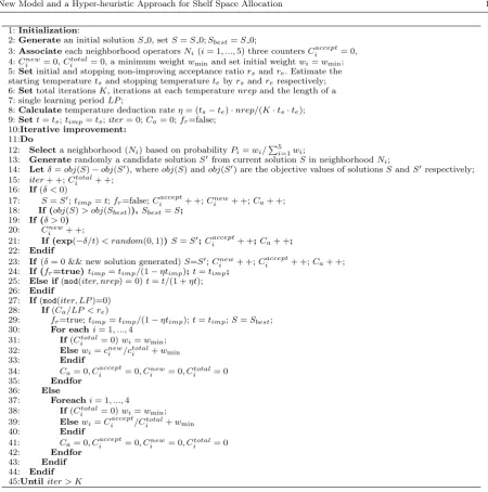
1:Initialization:
2:Generatean initial solutionS0, setS=S0;Sbest=S0;
3:Associateeach neighborhood operatorsNi(i= 1, ...,5) three countersCiaccept= 0, 4:Cnew
i = 0,Citotal= 0, a minimum weightwminand set initial weightwi=wmin; 5:Setinitial and stopping non-improving acceptance ratiorsandre. Estimate the starting temperaturetsand stopping temperaturetebyrs andrerespectively; 6:Settotal iterationsK, iterations at each temperaturenrepand the length of a 7: single learning periodLP;
8:Calculatetemperature deduction rateη= (ts−te)·nrep/(K·ts·te); 9:Sett=ts;timp=ts;iter= 0;Ca= 0;fr=false;
10:Iterative improvement: 11:Do
12: Selecta neighborhood (Ni) based on probabilityPi=wi/∑5i=1wi;
13: Generaterandomly a candidate solutionS′ from current solutionSin neighborhoodNi;
14: Letδ=obj(S)−obj(S′), whereobj(S) andobj(S′) are the objective values of solutionsSandS′ respectively; 15: iter+ +;Ctotal
i + +; 16: If(δ <0)
17: S=S′;timp=t;fr=false;Ciaccept+ +;Cinew+ +;Ca+ +; 18: If (obj(S)> obj(Sbest)),Sbest=S;
19: If (δ >0) 20: Cnew
i + +;
21: If (exp(−δ/t)< random(0,1))S=S′;Caccepti + +;Ca+ +; 22: Endif
23: If(δ= 0 && new solution generated)S=S′;Cnew i + +;C
accept
i + +;Ca+ +; 24: If (fr=true)timp=timp/(1−ηtimp);t=timp;
25: Else if(mod(iter, nrep) = 0)t=t/(1 +ηt); 26: Endif
27: If(mod(iter, LP)=0) 28: If(Ca/LP < re)
29: fr=true;timp=timp/(1−ηtimp);t=timp;S=Sbest; 30: For eachi= 1, ...,4
31: If(Ctotal
i = 0)wi=wmin; 32: Elsewi=cnewi /ctotali +wmin
33: Endif
34: Ca= 0, Ciaccept= 0, Cinew= 0, Citotal= 0
35: Endfor
36: Else
37: Foreachi= 1, ...,4 38: If(Ctotal
i = 0)wi=wmin; 39: Elsewi=Ciaccept/Citotal+wmin
40: Endif
41: Ca= 0, Ciaccept= 0, Cinew= 0, Citotal= 0
42: Endfor
[image:13.595.83.534.68.523.2]43: Endif 44: Endif 45:Untiliter > K
Fig. 2.Pseudo code of the proposed multiple neighborhood search algorithm (Bai et al., 2012).
5. Extension: no clustering constraint
As mentioned earlier, the inclusion of a cluster constraint (12) simplifies the problem in a sense that the
search can concentrate on a smaller search space. However, the solution procedures proposed in this paper
can be easily adapted to the problem without this cluster constraint. For the gradient approach, choosing
both the best shelf and item will be based on function (13) only. For the multi-neighbourhood approach, two
things need to change: a) feasibility check procedure will be relaxed accordingly. b) New neighourhood moves
can be introduced which reallocate some of facings to another shelf. The overall framework and the other
multi-neighbourhood approach, which could adapt to the changes in a business environment. However, this
may not be the case for some mathematical programming techniques.
6. Numerical Examples
In this section, we describe the empirical data available and then present some examples based on this data.
6.1 Empirical input data
We use empirical data on daily sales, product attributes and available shelf space obtained from a European
supermarket chain. We focused on dry groceries which are delivered from the retailers’ distribution center.
Median sales per SKU are observed to be around 3.8 customer unit/week. The merchandising categories
which were included in the datasets are similar to the categories reported in (Broekmeulen et al., 2007).
The experiment contained SKUs (Stock-Keeping-Unit) from 44 stores. Usually, promotions are done in the
stores using other shelf space allocations. Therefore, promotions are eliminated to obtain the true mean
and the standard deviation of the weekly sales. The supermarket chain reported the shelf capacity for each
store-SKU combination. Unfortunately, the chain did not have data on the exact position of the products
[image:14.595.107.507.492.601.2]on the shelves, nor did they report on the specific sales prices of the SKUs due to reasons of confidentiality.
Table 3.Problem instance with 6 items
βik
Itemi hi li pi smini smaxi αi βi 1 2 3 4 5 6
1 143 47 6.62 3 10 45.80 0.88 – -0.001 0.008 0 0 0
2 143 47 5.94 2 8 93.57 0.73 0.029 – 0.022 0 0 0
3 150 50 4.59 3 8 42.59 0.88 0.016 0.026 – 0 0 0
4 150 76 3.92 1 10 68.52 0.34 0 0 0 – 0 0
5 143 47 7.93 1 6 22.74 0.80 0 0 0 0 – 0
6 150 50 6.09 3 10 16.92 0.66 0 0 0 0 0 –
6.2 Two case studies
Due to data availability and commercial confidentiality limitations, only two instances, one small instance
(m= 3,n= 6) and one medium-sized instance (m= 5,n= 29), were extracted from the data. For simplicity,
they are denoted as Pn6 and Pn29. Detailed information of these two instances is provided in the Tables
3 and 4. The instances are based on a coffee category. Due to the limited data available, sales prices are
[image:16.595.108.506.423.559.2]drawn from the range [2.0,8.0] with even probabilities and cross elasticities were uniformly sampled within
[-0.03,0.03] for the top 10 SKUs (in sales). The elasticities for the other SKUs are set to be zero. Direct space
elasticitiesβi were estimated by simple linear regression based on the real-world data. As can be seen from
Table 7, most of direct space elasticities are in the range [0,1]. There are a few values outside this range
though. A negative value means that a big displayed stock may leads to a decrease in demand (sometimes, a
customer may associate poor quality or deficits with some large-stocked items). Some direct space elasticities
are larger than 1 which means that allocating extra space to these items would lead to a larger increase in
demand. Note that these estimated values are only valid within the corresponding facings ranges [smin
i , smaxi ].
Once the allocated facings exceed this bound, the estimated direct elasticity values become invalid. All the
other values were directly drawn from the real-world data.
Table 5.A comparison of solutions by different approaches for Pn6.
Gradient Multi-neighborhood Optimal Solution
Itemi xi si zi xi si zi xi si zi
1 7 7 0 5 10 1 5 10 1
2 4 8 1 4 8 1 4 8 1
3 8 8 2 8 8 0 8 8 0
4 2 4 1 1 2 1 1 2 1
5 3 6 1 6 6 2 6 6 2
6 3 3 0 4 4 2 4 4 2
Objective (Best/Mean)* 8188.97 8975.50/8897.75 8975.50
Deviation from Optimum 8.8% 0.9% –
Time (in sec.) <0.1 1.2 58.6
*The best and mean objective by the multi-neighborhood algorithm were based on 10 independent runs. Both the gradient approach and the complete enumeration approach always obtained the same solution.
Tables 5 and 6 present a comparison of solutions obtained by the gradient approach, the multi-neighborhood
approach and the complete enumeration approach. All the algorithms were run on a PC with a Pentium
IV 1.8GHZ CPU and 2GB RAM. Due to its stochastic nature, the multi-neighborhood approach was run
20 times for each problem instance (with the best solution and average objective value over 20 runs being
Table 6.Solutions obtained by the gradient method and the multi-neighborhood approach for Pn29.
Gradient Multi-neighborhood (MN2)
Itemi xi si zi xi si zi
1 6 1 12 6 12 1
2 8 3 8 2 2 3
3 8 4 16 8 16 1
4 10 2 10 10 10 2
5 8 2 8 8 8 2
6 3 3 3 3 3 3
7 5 4 10 10 10 2
8 6 0 6 6 6 1
9 10 1 10 10 10 4
10 4 1 8 3 3 0
11 4 0 4 4 4 4
12 8 3 8 8 8 3
13 3 2 3 3 3 0
14 6 2 6 6 6 2
15 7 3 7 5 10 4
16 2 2 2 1 2 1
17 6 0 6 6 6 0
18 2 4 2 1 2 1
19 4 4 8 8 8 3
20 4 1 8 8 8 0
21 6 3 6 3 6 1
22 1 2 1 3 3 3
23 1 2 1 1 1 0
24 4 0 4 2 4 1
25 4 4 8 4 8 1
26 5 0 5 4 4 4
27 5 4 5 6 6 0
28 1 2 1 8 8 3
29 3 4 6 4 8 4
Objectve (Best/mean)* 97134.70 110640.14/110007.113
Time (in sec.) <0.5 43.4
*The best and mean objective by the multi-neighborhood algorithm were based on 20 independent runs. The gradient approach always returned the same solution.
instance Pn6, it finds a solution in less than 0.1 seconds with an objective value that is 8.8% away from
the optimum. In contrast, the complete enumeration is quite slow, with a computational time of almost a
minute. For Pn29, the complete enumeration approach (embedded with some simple bounding heuristics)
failed even to find a feasible solution after 12 hours of computational time. The multi-neighborhood approach
seems to provide an appropriate compromise between the solution quality and the computational time. On
average, among 20 runs, it obtains a solution that is only 0.8% away from the optimum with much less
opti-mal solution among 20 runs. For the instance Pn29, the multi- neighborhood approach could obtain 12.3%
(= 11064097134.14−.9713470 .70) improvement over the gradient approach in terms of the objective function.
Neverthe-less, the multi-neighborhood approach consumes much more (but still reasonable) CPU time. A graphical
[image:18.595.72.540.183.521.2]representation of the best solution by the multi-neighborhood approach is given in the Fig. 3.
Fig. 3.The best solution obtained by the multi-neighborhood approach out of 20 runs
6.3 Sensitivity Analysis
Shelf space Although shelf space is an expensive resource, in some cases, retailers may be able to invest more
in space in order to increase sales. The question that retailers are interested in is how much extra sales can be
realized by investing in more shelf space. The small instance is considered here since its optimal solution can
be found reasonably quickly by the complete enumeration method. Fig. 4 plots the relationship between the
It can be seen that increasing shelf length has a positive effect on the sales. However, this relationship is
extremely nonlinear. For example, when the shelf length is increased from 300 to 340, the sales increased by
almost 15%. However, expanding the shelf length from 780 to 1000 does not increase sales at all. In general,
when the shelf space is very limited, an increase in the shelf space has a larger impact on the sales than
when the shelf space is already large. When the shelf length reaches over 1400, it no longer has an impact on
sales. This is partially due to the diminishing return demand function we used. In addition, the number of
facings allocated to the items may reach the maximum allowed upper bounds, which define the valid ranges
of the demand function.
0% 10% 20% 30% 40% 50% 60% 70%
300 500 700 900 1100 1300 1500
Shelf Length Lj
In
cr
ea
se
%
i
n
S
a
le
[image:19.595.204.404.271.423.2]s
Fig. 4.The impact of shelf space over sales.
Sensitivity of the parameter estimation error A number of parameters were estimated in the problem model.
For example, the scale coefficient (αi), the space elasticity (βi), and the cross elasticities (βik). This could
introduce some estimation errors into the model. In this section, we analyze the effect of these estimation
errors over the objective function. The small instance was used again due to its known optimal objective. The
sensitivity analysis method is similar to the approach used in (Borin and Farris, 1995). For each estimated
parameter set (αi,βi, orβik), a random error is added to each element of the considered parameter set. The
errors were sampled from a normal distribution with mean values set to 0. The errors have mean 0, while the
resulting parameters have means to be the true values and increasingly larger standard deviations. LetX%
be the mean absolute percent error from the true values. The enumeration search was again carried out to
obtain the global optimal objective values for both the original instance (without error) and the instance with
error,Me%, was calculated by|Morig−Merror|/Morig. For each parameter set, this process was repeated 50
[image:20.595.173.442.163.296.2]times. The average relative objective errors are presented in Table 7.
Table 7. Average impact of errors in parameter estimation.
αi βi βik
X% Me% X% Me% X% Me%
2.7% 1.28% 2.5% 2.31% 3.2% 1.52%
5.4% 2.57% 5.6% 4.61% 6.4% 1.49%
7.6% 3.80% 7.4% 7.59% 9.6% 1.53%
10.6% 5.48% 10.4% 7.03% 12.9% 1.63%
14.2% 6.61% 12.3% 9.37% 16.3% 1.54%
16.8% 7.14% 15.2% 11.67% 18.9% 1.82%
17.7% 13.76% 16.0% 16.94% 23.0% 1.82%
21.2% 10.64% 17.4% 12.69% 26.0% 1.67%
22.4% 12.13% 20.5% 12.19% 27.0% 1.83%
X%: Mean absolute percent error in parameter estimation
Me%: Mean percent deviation from optima
0% 5% 10% 15% 20% 25% 30% 35% 40% 45%
0% 5% 10% 15% 20% 25%
Parameter Error X%
E
r
r
o
r
%
i
n
S
a
le
[image:20.595.205.409.374.526.2]s
Fig. 5.Distribution of errors in sales with respect to errors inαi
Figs. 5, 6, 7 plot the distributions of the resulted errors in sales with respect to the errors in three
parameter sets: αi, βi, and βik. Each square box represents a given percentage error in sales. Hence, areas
crowded with square boxes mean more values appearing in that range. The solid line plots the trend of the
average relative error in sales across different parameter errors. The evidence suggests that the model is
reasonably robust. In general, average errors in sales range from 1.28% to less than 17%. Larger errors in
parameter estimation generally result in larger errors in sales prediction by the model, except for the cross
0% 5% 10% 15% 20% 25% 30% 35% 40% 45%
0% 5% 10% 15% 20% 25%
Parameter Error X%
E
r
r
o
r
%
i
n
S
a
le
[image:21.595.206.412.95.246.2]s
Fig. 6.Distribution of errors in sales with respect to the errors inβi
0% 1% 2% 3% 4% 5% 6% 7%
0% 5% 10% 15% 20% 25% 30%
Parameter Error X%
E
r
r
o
r
%
i
n
S
al
e
s
Fig. 7.Distribution of errors in sales with respect to the errors inβik
Cross elasticities have least impact on the sales. This is probably due to the fact that their values are much
smaller compared withαi andβi.
6.4 Larger instances
In order to fully test the model and the solution methods, we generated two artificial data sets (Set1 and Set2),
each of which is comprised by 20 larger instances. The parameters that are used to create these instances
are the same to those used by Hwang et al. (2009). Each instance in Set1 contains 50 items and 5 shelves
(denoted as n50m5 n50m5 10). Instances in Set2 have 100 items and 10 shelves (denoted as n1000m10
01-n100m10 10). These instances are publicly available for download from
[image:21.595.204.407.289.440.2]Two versions of the simulated annealing hyper-heuristics were implemented and tested. In the first version
(denoted as MN1), the neighborhoods are uniformly selected and hence does not have any adaptation. The
second version is the one that we described in Fig. 2 where the probabilities of neighborhood calls are
adaptively tuned during the search. All the other parameters for MN1 and MN2 are the same. In addition,
we also implemented a first-decent variable neighbourhood search (VNS), consisting of two repetitive phases,
local search phase and perturbation phase. The neighborhoods N1, N2, N3, N4 described in section 4.2.1
were used as the first-descent local search neighborhoods and N5 was used as a perturbation method. The
VNS algorithm successively searches through each of the local search neighborhoods (i.e. N1-N4) until it
gets stuck at a local optimum. A perturbation is then applied to the current solution using neighborhood
function N5 before the next iteration of the local search phase.
The following parameter settings were used: for both MN1 and MN2, we set K = 2×10⁶, LP = 5000,
which corresponds to around 280 seconds computational time for Set1 instances and 600 seconds for Set2
instances on the same machine that we used in the previous experiments. For VNS, computational time limit
was set to 280 seconds for Set1 instances and 600 seconds for Set2 instances. Therefore, all the algorithms
used approximately similar amount of computational time. Each of the 20 instances was solved by each of
Table 8 gives the computational results for these 20 instances by the gradient method, the variable
neighborhood search (VNS), the multi-neighborhood approach with random neighborhood selection (MN1),
multi-neighborhood approach with adaptive neighborhood selection (MN2). A few observations can be made
from the results; 1) The gradient method performed poorly, particularly for instances with 100 items and 10
shelves. 2) The variable neighbourhood search (VNS) does well for Set1 instances but are significantly inferior
to MN1 and MN2 for instances in Set2. 3) In terms of average objective values, the hyper-heuristic approach
with adaptive neighbourhood selection (MN2) performed generally better than the random neighbourhood
selection (MN1). Nevertheless, the mean results by MN1 were better for 4 instances (e.g. n50 08, n100 02,
n100 08, n100 10).
The two-tailed student’s t-tests were also carried out to find out whether the proposed hyper-heuristic
method (MN2) is statistically different from VNS or MN1. Table 9 presents the probabilities of the test
results. We can see that, at 5% confidence level, MN2 is significantly different from VNS for every instance.
From both Table 8 and Table 9, we can conclude that MN2 is significantly better than VNS except for 3
out 20 instances (n50m5 07, n50m5 08, and n50m5 10), for which VNS performed better. The differences in
performance between MN1 and MN2 are not as obvious but overall MN2 is slightly better. For 8 out of 20
instances, there is no significant difference between them. For the remaining 12 instances, MN2 is significantly
[image:24.595.86.525.463.598.2]better than MN1 for 11 instances and MN1 outperformed MN2 statistically for 1 instance, n100m10 10.
Table 9.The probability results of the student’s t-tests between MN2, VNS and MN1.
Set1 MN2 vs VNS MN2 vs MN1 Set2 MN2 vs VNS MN2 vs MN1
n50m5 01 2.4% 4.2% n100m10 01 0.0% 40.7%
n50m5 02 0.0% 0.8% n100m10 02 0.0% 80.7%
n50m5 03 4.5% 0.2% n100m10 03 0.0% 3.6%
n50m5 04 0.0% 0.0% n100m10 04 0.0% 2.9%
n50m5 05 0.0% 0.2% n100m10 05 0.0% 78.4%
n50m5 06 0.0% 1.1% n100m10 06 0.0% 62.5%
n50m5 07 0.0% 10.2% n100m10 07 0.0% 88.4%
n50m5 08 0.0% 3.2% n100m10 08 0.0% 52.3%
n50m5 09 0.0% 18.8% n100m10 09 0.0% 1.4%
n50m5 10 1.7% 0.0% n100m10 10 0.0% 4.8%
6.5 Adaptation of neighborhood selection
In our proposed algorithm, the selection of neighborhoods are based on an online learning mechanism.
23% 25% 27% 29%
b
o
rh
o
o
d
C
a
ll
s
N1
N2
15% 17% 19% 21%
43.5 38.5 34.6 31.4 28.7 26.5 24.6 22.9 21.4 20.2
P
e
rc
e
n
ta
g
e
o
f
N
e
ig
h
b
Temperature
N3
N4
N5
[image:25.595.150.465.90.325.2]Temperature
Fig. 8.Adaptation of neighbourhood calls at different annealing temperatures (For instance n50m5 01. Distributions for other instances are similar.)
performance than the random uniform neighborhood selection for most instances. Fig. 8 shows a typical
dynamic adaptation process of different neighbourhood calls over different annealing temperatures. It can be
observed that, although the probabilities with which neighborhoods were chosen are the same at the beginning
of the search, they are changed for different temperatures during the search. Overall, the first neighbourhood,
N1, was selected more than the other neighborhoods. This trend intensifies when the annealing temperature
decreases.
7. Conclusions
In this paper, we have presented a two-dimensional shelf space allocation model. The contributions of the
paper are two folds: 1) rather than focusing on a single dimension, shelf length, the proposed shelf space
allocation model adds the height dimension to the shelf space allocation decisions. As such, the new model
is much more realistic than one-dimensional models. 2) An efficient simulated annealing hyper-heuristic
approach is proposed for this 2D shelf space allocation problem. This approach can flexibly be adapted
to other types of shelf space allocation problems (e.g. three-dimensional versions) thanks to the increased
generality of hyper-heuristics compared to other heuristic methods. The performance of the algorithm were
We have showed via a small example used in a previous study, that explicitly taking into account the
height dimension will improve shelf space utilization and the resulting sales. Sensitivity analysis has shown
the benefits of the proposed algorithm: if one has allocated limited shelf space to an SKU, a shelf space
increase will have a relatively large impact on sales than if one already has abundant shelf space allocated.
In addition, the shelf space allocation model is fairly robust against input parameter errors.
References
R. Bai and G. Kendall. An investigation of automated planograms using a simulated annealing based hyper-heuristics. In
T. Ibaraki, K. Nonobe, and M. Yagiura, editors,Metaheuristics: Progress as Real Problem Solvers, volume 32 ofOperations
Research/Computer Science Interfaces, pages 87–108. Springer, 2005.
R. Bai and G. Kendall. A model for fresh produce shelf space allocation and inventory management with freshness condition
dependent demand.INFORMS Journal on Computing, 20(1):78–85, 2008.
R. Bai, E. K. Burke, and G. Kendall. Heuristic, meta-heuristic and hyper-heuristic approaches for fresh produce inventory
control and shelf space allocation. Journal of the Operational Research Society, 59:1387–1397, 2008.
R. Bai, J. Blazewicz, E. K. Burke, G. Kendall, and B. McCollum. A simulated annealing hyper-heuristic methodology for
flexible decision support.4OR - A Quarterly Journal of Operations Research, 10:43–66, 2012.
N. Borin and P. Farris. A sensitivity analysis of retailer shelf management models.Journal of Retailing, 71(2):153–171, 1995.
N. Borin, P. W. Farris, and J. R. Freeland. A model for determining retail product category assortment and shelf space
allocation.Decision Sciences, 25(3):359–384, 1994.
R. A. C. M. Broekmeulen, J. C. Fransoo, and K. H. van Donselaar T. van Woensel. Shelf space excesses and shortages in
grocery retail stores. Technical report, Eindhoven University of Technology, The Netherlands, 2007.
E. K. Burke, E. Hart, G. Kendall, J. Newall, P. Ross, and S. Schulenburg. Hyper-heuristics: An emerging direction in modern
search technology. In F. Glover and G. Kochenberger, editors,Handbook of Metaheuristics, pages 457–474. Kluwer, 2003a.
E. K. Burke, G. Kendall, and E. Soubeiga. A tabu-search hyperheuristic for timetabling and rostering. Journal of Heuristics,
9(6):451–470, 2003b.
E. K. Burke, S. Petrovic, and R. Qu. Case based heuristic selection for timetabling problems. Journal of Scheduling, 9(2):
115–132, 2006.
E. K. Burke, B. McCollum, A. Meisels, S. Petrovic, and R. Qu. A graph-based hyper heuristic for educational timetabling
problems.European Journal of Operational Research, 176(1):177–192, 2007.
M. Corstjens and P. Doyle. A model for optimising retail space allocations. Management Science, 1981.
K. Cox. The effect of shelf space upon sales of branded products.Journal of Marketing Research, 7:55–58, 1970.
R. Curhan. The relationship between space and unit sales in supermarkets.Journal of Marketing Research, 9:406–412, 1972.
K. A. Dowsland, E. Soubeiga, and E. K. Burke. A simulated annealing based hyperheuristic for determining shipper sizes for
storage and transportation. European Journal of Operational Research, 179(3):759–774, 2007.
X. Dreze, S. J. Hoch, and M. E. Purk. Shelf management and space elasticity. Journal of Retailing, 70(4):301–326, 1994.
F. Glover and G. A. Kochenberger, editors. Handbook of Metaheuristics. Springer, 2003.
David Goldberg. Genetic Algorithms in Search, Optimization and Machine Learning. Addison Wesley, 1989.
E. Hart, P. Ross, and J. A. Nelson. Solving a real-world problem using an evolving heuristically driven schedule builder.
Evolutionary Computing, 6(1):61–80, 1998.
H. Hwang, B. Choi, and M.-J. Lee. A model for shelf space allocation and inventory control considering location and inventory
level effects on demand. International Journal of Production Economics, 97(2):185–195, 2005.
Hark Hwang, Bum Choi, and Grimi Lee. A genetic algorithm approach to an integrated problem of shelf space design and item
allocation.Computers & Industrial Engineering, 56:809–820, 2009.
J. Kotzan and R. Evanson. Responsiveness of drug store sales to shelf space allocations. Journal of Marketing Research, 6:
465–469, 1969.
A. Lim, B. Rodrigues, and X. Zhang. Metaheuristics with local search techniques for retail shelf-space optimization.Management
Science, 50(1):117–131, 2004.
Chase C. Murray, Debabrata Talukdar, and Abhijit Gosavi. Joint optimization of product price, display orientation and
shelf-space allocation in retail category management. Journal of Retailing, 86:125C136, 2010.
P. Ross. Hyper-heuristics. In E. K. Burke and G. Kendall, editors,Search Methodologies: Introductory Tutorials in Optimization
and Decision Support Techniques, chapter 17, pages 529–556. Springer, 2005.
K. Sastry, D. Goldberg, and G. Kendall. Genetic algorithms. In E.K. Burke and G. Kendall, editors,Search Methodologies:
Introductory Tutorials in Optimization and Decision Support Techniques, pages 97–125. Springer, 2005.
T. Urban. An inventory-theoretic approach to product assortment and shelf-space allocation.Journal of Retailing, 74(1):15–35,
1998.
T. Van Woensel, R.A.C.M. Broekmeulen, K.H. van Donselaar, and J.C. Fransoo. Planogram integrity: a serious issue. ECR
Journal, 6:4–5, 2006.
M.-H. Yang. An efficient algorithm to allocate shelf space.European Journal of Operational Research, 131:107–118, 2001.
F. Zufryden. A dynamic programming approach for product selection and supermarket shelf-space allocation. Journal of