Genetic characterisation and social structure of the East Scotland population of bottlenose dolphins (Tursiops truncatus)

(1)

GENETIC CHARACTERISATION AND SOCIAL STRUCTURE OF THE EAST SCOTLAND POPULATION OF BOTTLENOSE

DOLPHINS (TURSIOPS TRUNCATUS)

Valentina Islas-Villanueva

A Thesis Submitted for the Degree of PhD at the

University of St Andrews

2010

Full metadata for this item is available in Research@StAndrews:FullText

at:

http://research-repository.st-andrews.ac.uk/

Please use this identifier to cite or link to this item:

(2)

Genetic Characterisation and Social Structure of

the East Scotland population of bottlenose

dolphins (

Tursiops truncatus

)

Valentina Islas-Villanueva

Submitted for the degree of Doctor of Philosophy to the University of St Andrews

September, 2009

(3)

In submitting this thesis to the University of St Andrews we understand that we are giving permission for it to be made available for use in accordance with the regulations of the University Library for the time being in force, subject to any copyright vested in the work not being affected thereby. We also understand that the title and the abstract will be published, and that a copy of the work may be made and supplied to any bona fide library or research worker, that my thesis will be electronically accessible for personal or research use unless exempt by award of an embargo as requested below, and that the library has the right to migrate my thesis into new electronic forms as required to ensure continued access to the thesis. We have obtained any third-party copyright permissions that may be required in order to allow such access and migration, or have requested the appropriate embargo below.

The following is an agreed request by candidate and supervisor regarding the electronic publication of this thesis:

Embargo on both all or part of printed copy and electronic copy for a fixed period of 1 year (maximum five) on the following ground:

publication would preclude future publication;

(7)

Acknowledgments:

I have dedicated my previous theses to my mother as I dedicate the few good things that I have done. Although thanks to her effort I have managed to achieve all the little steps that have lead me to this point; I think this time she has to share the dedication of this work with both my supervisors. If I would have to remember the whole 4 years of my PhD with just one memory, it would be my morning meetings with both of them; fifteen minutes before Vincent’s arrival you could see me and Jeff running around computers and printers to put some recently cooked figures in front of Vincent’s eyes at sharp 9 am. If you could put Jeff and Vincent into a blender you could simply achieve perfection. Jeff and his lovely family provided me with the support and the warmth of a family when mine was far away. During my 4 years in this office, Jeff would always stop whatever he was doing to listen to my absurd theories and help me with my analyses and this project would have simply not been accomplished if it wasn’t for Vincent perseverance. He managed to pushed me beyond my limits always being supportive and interested in the development of my career. I will also always be grateful to him for the great opportunity he gave me, to work with such an amazing population of dolphins. Among all the famous

bottlenose dolphins in the world, the East Scottish population is a top celebrity and I feel infinitely lucky to have been able to study them and carried out fieldwork in such a beautiful and wild place. Thank you very much to both of you!

I would like to thank Bob Reid, Scottish Strandings Coordinator and Paul Jepson, Marine Mammal Strandings Research Coordinator of the Institute of Zoology in London, for their time and attention in providing the strandings samples for this study.

To my examiners: Prof. Mike Ritchie and Dr. Michael Kruetzen.

To all the people that kindly helped me with lab, fieldwork or computer crisis: Nicky Quick, Gordon Hastie, Gordon Brown, Pati Celis, Kati Michalek. Jon Ashburner, Stephanie King, Simon Moss, Maria Keays, Murray Coults, Sean Earnshaw, Dave Forbes , Luke Rendell, Daniel Barker, Adrian B. Sonja H., Willemijn Spoor, Barbara Cheeney, Christoph E.and Saif

Special thanks to Lianne Baker for always facilitating things within the University and to Tanya Snedon the best technician in the world!

To my present and past office and labmates but especially to the ones that had to suffer my severe unfriendliness during the last months of my PhD: Maria, Elina, Gil, Andrew, Anna, Vicky, Paty, Gordon and Joe.

Thank you very much to: Stephanie King, Andy Foote and Nicky Quick for the challenging task of making some sense out of my paragraphs and correcting my very crappy English.

No huge task can be completed without a network of wonderful people that make you laugh, wipes your tears, feeds you and get you drunk whenever is needed, and supports you unconditionally, to my friends: Stephanie, Emma, Alex, Katie, Amy, Maria K, Maria H, Laura D, Anna S, Louise C, Willemijn, Thomas G, Sarah and John, Catherine and Hugh, CJ , Pete and Carmel, Rodrigo Villagra, Martina, Argelia, Iliana, Lorena C and Lore Viloria, Rodolfo Salas, Carlos de Luna, Andy F, Daniel Pinero, Nathan B., Paty, Gordon, Oli, Luko and the Music Quiz!. Thanks to the unconditional and constant support of my sister, Francina and my lovely family in Sweden and Mexico.

(8)

St Andrews

I love how it comes right out of the blue

North Sea edge, sunstruck with oystercatchers.

A bullseye centred at the outer reaches,

A haar of kirks, one inch in front of beyond.

(9)

Genetic characterisation and social structure of the Eastern Scotland population of bottlenose dolphins (Tursiops truncatus)

Summary

The Eastern Scottish population of bottlenose dolphins (Tursiops truncatus) is the northernmost population of this species. The resident core of this

population consists of 120 to 150 different individuals. This small size and its geographical isolation from other populations raises questions about its

viability and whether the population has behavioural patterns that differ from those common to other populations of the same species. Microsatellite genetic diversity was low and mitochondrial DNA genetic diversity values were lowest in East Scotland compared to other populations worldwide and to neighbouring populations around UK waters. It has been well

documented, from four different field sites worldwide, that male bottlenose dolphins form alliances with preferred male associates. These alliances can last for several years and the males involved males show association

(10)

Chapter l Introduction:

1.1. Genetic consequences of social organization

Natural populations are generally structured in subpopulations

interconnected by different levels of migration (Perrin & Mazalov 2000). Gene flow is the main force that determines subpopulation structure and how independently they evolve from each other (Slatkin 1987). For gene flow to occur between two populations, they need to overlap in their distribution, while being sexually active and receptive to each other (Slater & Halliday 1994). These actions must be mediated by exchanging signals to attract mates; sometimes mates are chosen to be from the same population and sometimes they are from a distant one (Slater & Halliday 1994).

Individuals can gain ‘inclusive fitness’ through the reproduction of related individuals as well as through their own reproduction (Hamilton 1963); (Maynard-Smith 1964). This idea supports behaviours such as altruism, aggression, cooperation, selfishness and spite (Griffin & West 2002). If a particular gender is philopatric, individuals of this population will spend more time with their close relatives, which will allow kin selection to operate on social behaviours (Maynard-Smith 1964).

(11)

In a highly inbred population, females would suffer the costs of inbreeding depression by investing their resources in non-viable offspring. Under this scenario, they would be more likely to choose, when possible, migrant mates, instead of local ones, thus forcing local males to disperse (Lehmann & Perrin 2003). Amos et al. (2001) showed that certain species of marine mammals could avoid inbreeding by selecting mates that are highly dissimilar to themselves. Another possibility could be that as females suffer more in an inbred population they would be expected to disperse (Waser et al. 1986).

These behavioural differences have obvious implications in the population structure of mammals. Maternal stable relationships are important in African elephants (Loxodonta africana); they live in fission-fusion groups with core groups of females comprised by first order relatives (Archie et al. 2008). The strong associations of female relatives and male dispersal are also common in rhesus monkeys (Macacca mulata) (Melnick 1987; Widdig et al. 2006). On the other hand maternal relatedness does not seem to affect strong female associations in bonobos (Pan paniscus) (Hashimoto et al. 1996) or male affiliations in chimpanzees (Pan troglodytes) (Goldberg & Wrangham 1997; Mitani et al. 2000). In Baboons the differences in reproductive success between males and their short term dominant state, result in a population that is sub-structured in age groups of paternal relatives (Altmann et al. 1996).

1.2. Social structure in Odontocetes

The ordercetaceais subdivided into the mystecetes (baleen whales) and the odontocetes (toothed whales, dolphins and porpoises) (Rice 1989a).

(12)

macrocephalus), pilot whales (Globicephala melas) and bottlenose dolphins (Tursiops spp). All these show a variety of complex patterns of association and relatedness that will be briefly described below.

Killer whales off southwest Canada live in sympatric populations that have been named resident and transient. Resident killer whales feed primarily on fish and live in matrilineal groups where males and females do not disperse, they gather with other matrilineal groups forming pods. Transient killer whales feed on other marine mammals and they also gather in matrilineal groups of small size that require dispersal from the natal group (Baird 2000).

Sperm whales are also grouped in female matrilines of around 10 individuals that are kin related which associate with other groups for a certain amount of time (Richard et al. 1996). Male sperm whales on the other hand leave their natal groups to join ‘bachelor’ groups. As they grow larger they become more solitary and migrate to higher latitudes (Rice 1989b). Pilot whales (Globicephala melas) also associate with kin and they form very stable family bonds. It seems that both mature males and females stay in their natal pods throughout their lives but males only reproduce with females form other pods (Amos et al. 1993).

Bottlenose dolphins (Tursiops spp) show a variety of complex social

(13)

associates (Smolker 1992), in others they form female bands of close relatives (Wells et al.1987) and in others they can be found in groups of similar

reproductive state (Möller & Harcourt 2008). Male-female relationships seem to be restricted to mother– calf pairs or to sexual interactions (Connor et al. 2000b).

1.3. The species studied

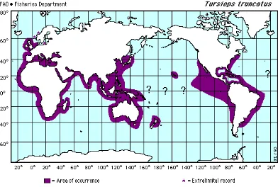
The bottlenose dolphinTursiops truncatus(Montagu, 1821), is a well known and studied odontocete species. It shows a worldwide distribution and its presence is greater in coastal regions of tropical and temperate waters (Shane 1988), though they also inhabit pelagic habitats (Jefferson et al. 1996) (fig. 1).

Besides its presence in the United Kingdom and the north of Europe, it is almost always found in latitudes between 45º north and south (Jefferson et al. 1996).

In the Atlantic Ocean it occurs in the northern Gulf of Mexico, Georges Bank off Massachusetts, the British Isles, the Baltic Sea including the Gulf of

Finland, the Mediterranean and Black seas, Newfoundland and Norway (Rice 1998). Its presence has been well documented down to the southern Gulf of Mexico, the Mexican Caribbean (Delgado-Estrella 2002) and Belize (Bilgre et al. 1995).

In the Pacific the distribution ranges north to the Bo Hai, East China Sea, central Honshu, Kure Atoll, Hawaii, Isla Guadalupe (Rice 1998), the inner Gulf of California (Ballance 1990), Monterey Bay in California to Puget Sound in Washington State. In the Southern Hemisphere it occurs south to Golfo San Matias in Argentina, 18ºS in northern Namibia, Port Elizabeth in Cape

(14)

of Australia including Tasmania, South Island (Rice 1998) and Doubtful Sound (Williams et al. 1993) in New Zealand, and Concepción, Chile (Rice 1998).

[image:14.595.93.485.302.566.2]

Populations all over the species worldwide distribution show different behavioural specializations and different phenotypes. These differences are related to local adaptations or a particular social structure but it is not clear if they reflect real phylogenetic separations or just a great phenotypic plasticity (Curry & Smith 1997).

Figure 1. Tursiops truncatusworldwide distribution according to Jefferson et al. 1996.

1.4. The studied population

(15)

that bottlenose dolphins were not common in the Moray Firth until the very end of the 17th_century.

Up in the Moray Firth the presence of bottlenose dolphins has been documented all year round with high density peaks in the summer. By traditional photo-identification techniques, 115 individuals have been identified as residents. The group size can fluctuate from 2-46 with an

average of 6.45 and it is correlated to the amount and distribution of the prey (Wilson 1995). Outside the Moray Firth surveys around Aberdeen harbour have documented the presence of bottlenose dolphins mostly displaying foraging behaviour (Sini et al. 2005). Its presence around Fife Ness seems to be restricted to the summer period and at least 65 individuals have been identified, although the population could be composed of up to 130 different individuals (Quick2006).

Bottlenose dolphins show different association patterns. They can form long lasting behavioural associations, or short acquaintances that can last a few days (Gero et al. 2005). The individuals in the Moray Firth do not show any strong, long lasting association, males seem to associate with different

individuals of both sexes more often than females do and tend to form bigger groups (Wilson 1995). On a bigger scale this population appears to be

stratified in two groups that use the same habitat at different times,

suggesting some kind of competition between social groups or communities (Lusseau et al. 2006; Wilson et al. 1997a) connected via a limited number of individuals (Lusseau et al. 2006).

Population structure studies of dolphins inhabiting UK waters suggest that the Moray Firth population is isolated from its neighbouring populations (Nichols et al. 2007; Parsons et al. 2002), but is genetically closer to the

(16)

Firth population were much lower than the ones of the other UK populations and other populations around the world (Parsons et al. 2002).

This decrease in genetic diversity and the isolation and small size of the East Coast Scottish population, raises concerns about the possibility of inbreeding depression that could have detrimental effects. Wilson et al. (1997b) found that 95% of the dolphins sampled in four years showed some kind of skin lesion and 6% showed deformities; these lesions were more extensive in female adults and calves than in male adults. When studying several populations with skin lesions worldwide, there was no correlation between these lesions and contaminant levels the populations is exposed to, but there was a correlation with low temperature and low salinity (Wilson et al. 1999). This suggests that the habitat these animals occupy can cause physiological stress that makes the population vulnerable (Wilson et al. 1999).

Populations around the UK occupying the extreme range of the distribution of the species seem to be under physiological stress; they have a small

population size and seem to show local adaptations. To what extent are these facts a cause of concern? Nichols et al. (2007) investigated the genetic origins and population structure of a group of bottlenose dolphin bones found in the Northeast of England (Flixborough). These individuals showed the dominant mitochondrial haplotype of the Eastern Scottish population, but they were differentiated as a population by microsatellites (Nichols et al. 2007). Nichols et al. (2007) suggested that local habitat dependence is related to regional genetic structure in these populations. The fact that the Flixborough

(17)

1.5. Methodological considerations 1.5.1 Phylogeography

Phylogeography is a field that studies the geographic distribution of the genealogical lineages of different species (Avise 2000). It studies the time and space of several genes of interest that may be used to know the actual

distribution and genetic structure observed in natural populations. The analysis and interpretation of lineage distributions requires the integration of several fields like population genetics, molecular genetics, ethology,

demography, phylogenetic biology, paleontology and historical geography (Avise 2000).

Population genetics has grown widely in the last 15 years due to the introduction of new DNA based technologies. Sequence analysis of

mitochondrial DNA (mtDNA) and the identification of nuclear microsatellite genotypes have become two standard tools in most of the animal genetic research, since they allow us to make inferences of phylogenetic relationships, gene flow, phylogeographic patterns and genetic variability (microsatellites and mtDNA), as well as fine analyses of population structure (microsatellites) (Sundqvist et al. 2001).

1.5.2. Mitochondrial DNA (mtDNA)

(18)

its substitution rate may be three to five times higher than the rest of the mitochondrial genome (Avise 2000). The substitution rate for cetaceans compared to humans seems to be one degree of magnitude lower, but similar to interspecific rates shown in primates and rodents(Hoelzel et al. 1991) (Hoelzel et al. 1991). Insertions and deletions are not as common in cetacean control regions as they are in other taxa. Point mutations seem to play the most important role in cetacean control region evolution (Hoelzel et al. 1991).

In spite of this high polymorphism the central position of the control region shows a similar nucleotide composition between different species and it does not diverge faster than the rest of the protein-coding genes of the

mitochondrial genome (Hoelzel et al. 1991). This feature makes inter and some intraspecific comparisons of the control region plausible and quite informative.

1.5.3. Nuclear genetic markers: Microsatellites.

Microsatellites also known as STR, SSR and SSLP (Short Tandem Repeats, Simple Sequence Repeats and Single Strand Length Polymorphisms) (Bruford & Wayne 1993; Tautz & Renz. 1984) are small DNA fragments widely spread in the eukaryotic genomes (Tautz & Renz 1984). These fragments consist of motifs of one to six nucleotides that repeat themselves in tandem up to 60 times or more (Goldstein & Pollock 1997). In eukaryotes these fragments can be found every 10 Kb in the DNA sequence and they constitute approximately 5% of the genome (Tautz 1989).

(19)

observe them in common polyacrilamide gels and detect small differences between them (Tautz 1989).

Microsatellites are extremely variable in the number of alleles reported due to the mutations in the number of repeated units by insertion or deletion (Tautz 1993 cited in: Nauta and Wissing 1996). The mutation rate of microsatellite lociis very high and seems to range between 10–5_{and –10}-2_{(Weber & Wong} 1993). This characteristic and the fact that they are relatively easy to screen have made them quite popular in population genetics, relatedness, parentage and individual identification studies (Goldstein & Pollock 1997).

These markers have become quite commonly used in cetacean research. Several studies have characterized nuclear microsatellites for their use in population studies (Valsecchi and Amos, 1996; Shinohara et al.1997; Rooney et al.1999; Hoelzel et al. 1998b; Krutzen et al. 2001). This makes it easier to find polymorphiclociin specific populations and gives us the opportunity to compare patterns in different locations from different studies. Most of the microsatellites in cetaceans have been developed to amplify dinucleotide motifs. Dinucleotide microsatellites scoring have been found to convey several mistakes while genotyping that result in large amount of errors in assigning paternity in wild populations (Hoffman & Amos 2005) mainly due to the presence of stuttering bands that are a common by-product of PCR amplification (Litt et al. 1993). For these reasons tetranucleotide markers are now becoming more widely used in the recent years and a couple of studies have developed them for cetaceans (Coughlan et al. 2006; Nater et al. 2009). Nater et al. (2009) developed a set of 19 tetranucleotide markers for bottlenose dolphins and compared their accuracy to previous dinucleotide

(20)

Aims of my PhD study:

The main aim of my PhD study was to investigate how the social patterns of bottlenose dolphins in the East Scottish population of bottlenose dolphins would be affecting the genetic patterns observed in the same. To achieve this objective I obtained biopsy samples and photo-identification data from the East Scottish population of bottlenose dolphins during the summer periods of 2006 and 2007.

I employed molecular techniques to confirm the sex of each sample and to investigate relatedness between the biopsied individuals. The association patterns of the East Scottish population were described including data from previous studies and a correlation between association and relatedness was investigated. The presence of strong bonds between female relatives in

cohesive groups along with the presence of adult male alliances was expected. Male alliances are a common reproductive strategy that has been documented in other populations of bottlenose dolphins around the world. Contrary to our expectations no correlations were found between association and relatedness (Chapter 3) and male alliances are not present in the population (Chapter 2).

(21)

Chapter 2 Population Structure of bottlenose dolphins

around UK waters.

2.1 Introduction:

Natural populations are generally structured in subpopulations,

interconnected by different levels of migration (Perrin & Mazalov 2000). Gene flow is the main force that determines subpopulation structure and how independently they evolve from each other (Slatkin 1987). An understanding of this structure is essential to create effective population management and conservation policies (O’Corry-Crowe et al. 1997), since subpopulations can be separated by varying degrees of genetic isolation. Traditional population genetic studies have employed genetic markers to uncover the dispersal dynamics of the population and how this is reflected in the population structure.

The study of genetic subdivision patterns among cetaceans is difficult because cetaceans are capable of traveling long distances (Escorza-Treviño & Dizon 2000) and have large habitat ranges with no evident barriers to gene flow besides water temperature, marine topography, (Würsig & Würsig 1979) productivity and surface features such as salinity (Natoli et al. 2005).

Bottlenose dolphins,Tursiops truncatus(Montagu 1821) along with other odontocete species show a promiscuous breeding system (Wells & Scott 1999). In the promiscuous or polygynous breeding systems the male’s reproductive success is limited by the availability of females, while the fitness of the

(22)

Patterns of dispersal are well differentiated between the sexes in a variety of organisms (Greenwood 1980). Although male biased dispersal is common in mammals and has been studied for several cetacean species with molecular markers (Escorza-Treviño & Dizon 2000; Lyrholm et al. 1999; Moller & Beheregaray 2004; O´Corry-Crowe et al. 1997), recent studies of bottlenose dolphins have found that both sexes can be phylopatric to some extent, showing fine scale structure related to water temperature, salinity and productivity (Natoli et al. 2005).

Among cetaceans intraspecific differentiation may be sympatric or parapatric (Hoelzel 1998). It seems that the main forces driving cetacean population differentiation are the specializations that result from their foraging behaviour (Hoelzel 1998). The evolution of these traits is influenced by three main

ecological aspects: place of birth, diet and foraging locations (Connor et al. 2000a) .

In bottlenose dolphin populations, two different ecotypes have been documented. In the Western North Atlantic “coastal” bottlenose dolphins have smaller sizes than the “pelagic” ones. Significant differences in measurements that are related to the size, mainly total length and skull length, were found between the two ecotypes, but with an extensive overlap in the measurements from both ecotypes (Mead & Potter 1995).

This pattern is reversed in the bottlenose dolphin populations of the Eastern North Pacific, where the morphological differences are so evident that coastal and pelagic dolphins have been considered to be different species. The

(23)

Hoelzel et al. (1998) used mitochondrial and nuclear genetic markers to find out to what extent these “coastal” and “pelagic” populations were genetically divergent in the North Atlantic. They found strong significant differences between the two ecotypes with both markers and a reduced genetic diversity among the “coastal” populations compared to the “pelagic” ones.

Pronounced genetic differences are not exclusive to foraging specializations in odontocetes. Dowling and Brown (1993) analysed RFLP´s (Restriction

Fragment Length Polymorphisms) for the mitochondrial DNA (mtDNA) control region ofTursiops truncatus, of neighbouring “coastal” populations and found significant differences between the stocks of the Atlantic Ocean and the Gulf of Mexico divided by the Florida Peninsula, but not between putative populations from the northeast of Florida or between populations from the southwest of Massachussets. More recently the population structure of resident “coastal” stocks from Sarasota Bay, Tampa Bay, Charlotte Bay and Matagorda Bay was analyzed using the control region of the mtDNA and nine microsatellite loci. Here, Sellas et al. (2005) found a strong population

subdivision with both markers for both sexes, indicating a strong phylopatry of males and females and a restricted gene flow between close, coastal, neighbouring populations.

(24)

philopatry of both sexes was also displayed by the populations of bottlenose dolphins from the Black Sea to the eastern North Atlantic, showing a

correspondence between the population structure and the use of habitat (Natoli et al. 2005).

Patterns of dispersal are well differentiated between sexes in a variety of organisms (Greenwood 1980). The resulting patterns of gene flow are of great importance to elucidate the phylogeographic pattern of the species (Avise 2000). Although the latter studies in bottlenose dolphins show philopatric patterns present in both sexes, male sex-biased dispersal has been

documented for several cetacean species by means of molecular analysis. This includes belugas, sperm whales and Dall’s porpoises (O’Corry-Crowe et al. 1997; Lyrholm et al. 1999; Escorza-Trevino and Dizon 2000) and bottlenose dolphin (Tursiops aduncus) populations of southeastern Australia (Möller & Beheregaray 2004).

A previous genetic study of the bottlenose dolphin populations of the United Kingdom, analysed mtDNA sequences from 29 stranded animals. This study revealed that the Moray Firth population was genetically closer to the

population of Wales than to the neighbouring population of the west coast of Scotland. The genetic diversity values of the Moray Firth population were much lower than the ones of other UK populations and other populations in the UK and worldwide (Parsons et al.2002).

(25)

the neighbouring populations with both mtDNA and microsatellites. They also found that the Flixborough population was mostly related to the East Coast population and other populations around the UK, but also much differentiated from them. They suggested that local adaptations in these populations that are located at the northern extreme of the distribution of the species are very strong and that the gene flow is much reduced.

In this study the largest set of cumulative samples to date from the

East Coast of Scotland and neighbouring populations was gathered. This collection included both stranded samples and biopsies from wild animals.

The aim of this study is to fine tune the relationships of the bottlenose dolphin populations around the UK. Previous studies have used only stranded

samples which origins could be inaccurate. They rather suffered of lack of sample size or they pooled together samples from different populations in order to achieve significance. In this study I try to establish if the East Coast of Scotland population is isolated from the neighbouring populations and to ascertain the implications that this may have on its conservation.

2.2 Methods:

2.2.1. Sample origins and DNA extractions

(26)

[image:26.595.91.457.72.607.2]

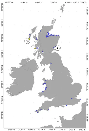
Figure 1. A map of Great Britain and Ireland showing the location of samples from strandings included in this study. Above the general area where the biopsies took place, the total number of biopsies is shown in circles. West Coast strandings in yellow circles are from individuals that shared the same haplotype with the Barra biopsies.

The total number of samples from the four putative populations is: a) East Scotland 69 individuals, b) West Scotland 19 individuals, c) Wales 15 individuals and d) English Channel 7 individuals.

(27)

Sixty-nine stranding samples came from tissue donated by the Scottish Strandings Coordinator in Inverness and the Marine Mammal Strandings Research Coordinator in London. Thirty-five biopsy samples from the East Coast of Scotland were collected as described in Chapter 3 and seven West Coast biopsy samples were collected only for purposes of genetic structure studies. The sex of the samples was given by the Stranding Network or determined with molecular techniques (Table 1) as described in Chapter 3.

Table 1. Details of one-hundred eleven samples collected in this study. Number and gender of the samples analyzed for the four populations.

Population

Strandings Biopsies Females Males Unknown

East Coast 35 35 24 41 5

West Coast 12 7 10 5 4

Wales 15 8 5 2

English Channel 7 4 3

Total

69 42 46 54 11

(28)

2.2.2. Mitochondrial DNA

A 660 bp section of the control region was amplified for 110 samples using the primers: Rev (5’GTGACGGGGCCTTTCTAA 3’) (LeDuc et al. 1999) and F2 (5’CTC ACC ACC AAC ACC CAA AG 3’). The F2 primer was designed with Primer 3 (http://primer3.sourceforge.net/) from aTursiops truncatus

sequence (AY963625) to obtain a longer fragment from the one already published by Parsons et al., (2002). Polymerase chain reaction conditions were as follow: 150µMdNTPs, 1.5 mMMgCl2, 20 mMTris-HCl pH 8.0, 50 mM KCl, 0.3 µMof each primer, 1.25 U/µL of Taq (Bioline) and 20 ng of DNA for a 25µL total reaction. PCR cycling profile: 4min at 95 °C, 30 cycles of 45 secs at 94°C, 1 min at 55.8°C and 1 min at 72 °C, followed by a final extension of 5 min at 72°C.

PCR products were purified with a QIAGEN QIAquick gel extraction kit and quantified for automated sequencing. Individuals were sequenced in both directions (forward and reverse)to verify the identity of each nucleotide in several cases where the sequences were not of high quality. Sequences were edited, checked and aligned by eye with BIOEDIT 7.0.5.3.

2.2.2.1 Genetic diversity

Nucleotide (π) and haplotypic (h) diversities (Nei 1987) were calculated for each population with the program ARLEQUIN 2.0 (Schneider et al. 2000). The population differentiation was measured with an analysis of molecular variance AMOVA (Excoffier et al. 1992) performed by Arlequin ver 3.1, along with the pairwise comparison of population differentiation indicesFST

(29)

2.2.2.2. Phylogeographical patterns

To organize the haplotypes observed in our populations in a way that portrays the evolutionary steps between them, a haplotypic network was created with the program TCS 1.18 (Clement et al. 2000). The assumption of this approach is that if an unknown mutation causing a phenotypic effect occurred at some point in the evolutionary history of the population, it would be embedded within the same historical structure represented by the

cladogram (Templeton et al. 1992). TCS calculates the frequencies of the haplotypes and creates a matrix of pairwise comparisons among them for which the probability of parsimony is calculated (Clement et al. 2000). The algorithm developed by Templeton et al. (1992) estimates all the possible cladograms with a high probability (>=0.95) of being true. The probabilities are higher when the number of changes between haplotypes is smaller and the probability decreases as the differences between haplotypes increase (Templeton et al. 1992). This method is suitable for intra-specific studies and it has been used to infer population genealogies particularly when they show low levels of divergence (Clement et al. 2000).

The different haplotypes across all the populations were compiled using the program COLLAPSE 1.2 (Posada © 1998-2006). These haplotypes were aligned withTursiops truncatushaplotypes obtained from GenBank

representing the following regions: Portugal (Tt-PO), Mediterranean (Med), Baltic Sea (BSea) and ENA (Eastern North Atlantic). Sequences from other species, were used as outgroups in the alignment, to resolve the relationships in a better way:Sousa chinensis(Schinensis),Stenella,Delphinus capensis

(30)

It has been suggested that when the evolutionary period represented by a cladogram is short, like it is in the case of intra-specific processes, maximum likelihood and maximum parsimony tend to give very similar results (Sober 1983 in Templeton et al. 1992). For this reason we constructed one tree with parsimony methods and another one with Bayesian ones. A parsimony consensus tree was constructed with PAUP (4.0 beta10) using 1000 bootstrap replicates andOrcinus orcaas the outgroup.

The individual haplotypes were analyzed to obtain a substitution model for the amplified region with the programs MODELTEST 3.05 (Posada &

Crandall 1998) and Modelgenerator v0.85 (Keane et al. 2006). The

substitution model that best fit the data according to Modeltest hierarchical likelihood ratio test and Modelgenerator Bayesian information criterion (BIC) was Trn+I+G (Tamura & Nei 1993). This model takes into account different rates of substitution between nucleotides: [A-C],[A-G],[A-T],[C-G],[C-T] and [G-T] (rate matrix) and different nucleotide frequencies. The rates among the sites are modeled using the gamma distribution. Thus a gamma parameter is required along with a proportion of invariable sites (I).

The probability of observing the data conditional to the phylogenetic model is the likelihood function, which is calculated assuming a model of character changes (Huelsenbeck & Ronquist 2001). The parameter for the likelihood model ‘lset’ was set as Nst=6, this model allows all the substitution rates to be different as is the case in the Trn+I+G model found in Modeltest. The model outcome had a proportion of invariable sites (I)= 0.6100, a gamma parameter of (G) = 0.5479 , a rate matrix= 1.0000 17.9388 1.0000 1.0000 40.1796.

(31)

samples. An autocorrelation test of the Ln function from the parameters obtained was carried out with the Statistical Program R (2005). The sampling of each tree was done every 20 000 generations. The initial

2 000 trees converged and were discarded (burnin), 2000000 generations were simulated with just one hot chain. The twoO. orcahaplotypes were

designated as outgroups.

2.2.3. Microsatellites

Twenty previously reported polymorphic nuclear microsatellite loci were analyzed for all 110 samples. The original source of the microsatellites and the PCR details are shown in Table 1 (Appendix). The twenty microsatellites were amplified with a fluorescent dye and automatically sequenced (Beckman Coulterer). The markers were amplified in 3 loci groups with a Multiplex PCR kit from (QIAGEN) with conditions shown in Table 2.

Table 2. Multiplex PCR Loci Groups Characteristics. Each Locus Group (LG) shows Locus

name, type of dye and concentration of dye are shown.

LG1

LG2

Locus

DYE [DYE] Locus

DYE [DYE]

TexVet5 D4 0.12 ρM Tur4_80 D4 0.16 ρM TexVet7 D3 0.8 ρM MK9 D2 0.8 ρM

D08 D3 0.6 ρM EV1 D3 0.8 ρM

D22 D4 0.12 ρM Tur_91 D4 0.16 ρM

MK6 D2 0.8 ρM Tur_117 D4 0.16 ρM

MK8 D4 0.08 ρM

LG3

Locus

DYE [DYE]

Tur105 D3 0.8 ρM

Dde72 D4 0.16 ρM

Tur138 D3 0.8 ρM

Dde84 D4 0.16 ρM

(32)

PCR reactions consisted of 10-20 ng of genomic DNA, 5 µl of Multiplex Mix and 3 µl of primer mix in a 10 µl reaction. The PCR profile was as follows: 95°C for 15 min followed by 30 cycles of 94°C for 30sec, 60°C for 90 sec and 71°C for 45sec, with a final extension of 72°C for 2 min.

Genotyping error was calculated separately for biopsies and strandings by randomly re-amplifying between 10% and 50% of the individuals for each locus. Each individual repeat was genotyped at least once and up to 6 times. If both allele lengths were identical each time, it was counted as two matches, but if either allele was different, it was considered two mismatches. The number of mismatches was divided by the total number of comparisons to obtain the error percentage for each locus in both biopsies and strandings. Finally all loci were run in Micro-checker (Van Oosterhout et al. 2004) to check them for null alleles, misgenotyping and stutter bands.

2.2.3.1. Genetic diversity

The genetic diversity was calculated as expected and observed heterozygosity (HEandHO) with the program (Genetix v 4.03). Deviation from HW

equilibrium and the probability test were calculated with GENEPOP v. 3.1d (Raymond & Rousset 1995b). The allelic richness was calculated with FSTAT 2.9.3.2 (Goudet 1995).

2.2.3.2. Population Structure

Pairwise comparisons of genetic differentiation (FST) were conducted with the program GENEPOP and FSTAT was used to test the significance of the

(33)

FSTis based to show high levels of differentiation when loci show high values of genetic diversity (high values of heterozygosity) and he developed a new measure to cope with that problem (DEST). DESTwas calculated with the program SMOGD (Crawford 2009) and compared with bothFST andRhoST. The linkage disequilibrium for each locus was calculated with GENEPOP. A sequential Bonferroni correction (Rice 1989c) was applied later to assess significance values.

The patterns of genetic structure were analyzed with Structure 2.3.1

(Pritchard et al. 2000). This program uses a Bayesian clustering analysis to determine the number of populations (K) observed according to the data and it determines the posterior probability of each single individual belonging to a particular population. The burn in period was set to 50 000 iterations and the probability estimates were determined using 1 000 000 Markov chain Monte Carlo (MCMC) iterations. Runs were conducted with K set from 1 to 10 with 10 runs for each value of K. Two separate tests were conducted with two different models: the no admixture model and the admixture model. The no-admixture model assumes that all the individuals come from the same

population K; this model is good at detecting subtle population structure. The admixture model assumes that the individuals from all the populations could have a common ancestor and it is good at dealing with hybrid zones. When running the admixture model we assigned individuals to five putative populations: Moray Firth, Outer Community, West Coast, Wales and English Channel, to confirm if the sampling area is informative. We divided the East Coast of Scotland in Moray Firth and Outer Community, to test if the

separation found by Lusseau et al. (2006), with a network analysis was

(34)

other locations. We did not divide the West Coast of Scotland samples due to the small number of biopsies from the region and the overall small sample size. Finally Structure was run with the admixture model, correlated frequencies, burnin of 11000, 1000000 repetitions and 5 iterations for each value of K from K=1 to K=8. This run included only the East Scottish samples to detect any structure within the population.

2.2.3.2.1. Estimation of parameter K

The power of the Bayesian algorithm to obtain the true K from the log probability of the data LnP(D), has not been well documented in a scenario with a non-homogeneous dispersal patterns. Evanno et al. (2005) developed a method to calculate anad hoc statistic called ΔK to correct this problem by

obtaining the second order rate of change of LnP(D) between the values of K.

This statistic (ΔK) can be obtained following 4 steps.

a) The means and standard deviation (SD) of the log probability for each

K 1 to 8 were obtained L′(K).

b) The first order rate of change was calculated as L″(K)= L(K)-L(K-1)

c) Absolute values of the second order rate of change were calculated as

/L″(K)/= /L′(K+1)- L′(K)/

d) ΔK was calculated as the absolute values of the second order rate of

change divided by the standard deviation of each K following the

following formula ΔK = L″K/SD L(K). The modal value of this

distribution is the true K.

2.2.3.3. Estimation of migration rates and sex biased dispersal

(35)

iterations, a sampling frequency of 2000 and burn-in of 999999 were the parameters for the analysis. The stabilization of the log likelihood values within the period set by the burnin was checked and the mean and variance of the posterior probabilities for the migration rates were obtained. Sex-biased dispersal was calculated with FSTAT by calculating pairwiseFST comparisons for females and males separately between all populations using 10,000 randomizations with a one-tailed test.

2.2.3.4. Relatedness between populations

As a final strategy to elucidate the relationship between the populations analyzed we used the Relatedness analyses explained in detail in Chapter 3. Pairwise symmetric relatedness was calculated for all the 101 individuals from the four populations analyzed with the program RE-RAT (Schwacke et al. 2005). Re-RAT calculated R using the Queller and Goodnight (1989) index with a jacknife over loci of 100 simulations. Average relatedness for each population and for classes of males and females were calculated in the same way.

A distance matrix was obtained by substracting 1 from each value of R for the pairwise comparison between individuals. With this distance matrix a

(36)

2.3. Results:

2.3.1. Mitochondrial DNA 2.3.1.1. Genetic diversity

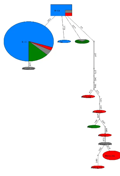
A 507 bp section of the control region of 87 samples from 4 populations was sequenced. The DNA in the remaining samples was too degraded to be sequenced. Twelve different haplotypes were found (Table 2). Between haplotypes 1, 2, 3, 5 and 7 there are just one or two differences, while the remaining haplotypes had multiple substitutions from haplotype 1.

Table 2. The twelve haplotypes. The position in the sequence where the substitutions occurred is shown in the top of the table, when the nucleotides remain the same it is indicated by a “-“.

Position 9 0 1 0 8 1 8 6 1 9 7 2 3 7 2 5 7 2 6 9 2 7 0 2 7 1 2 7 4 2 8 6 3 4 9 3 6 2 3 8 3 3 8 4 3 8 5 4 4 5 4 7 0

Hap1 C C T T C A T T C C C T C C A T T C Hap2 - - - T - - -

-Hap3 - - - T - - - T - - -

-Hap4 T - C C T - - C T - - - T - C - C

-Hap5 - G - - -

-Hap6 T - - C T - - C T - T - T - C - - T

Hap7 - - - G - - - T - - -

-Hap8 T - - C T - C C T - T - T - C - - T

Hap9 T - - C - - - C - - - - T T C - - T

Hap10 T - - C T - - C T - T C T - C C - T

Hap11 T - - C - - - C T - - - T - C - C

-Hap12 T - - C T - - C T - T - T - C - -

(37)

population) and Hap7. Animals from the English Channel had five different haplotypes in the six samples analyzed. Two of them were from Hap1 and one from Hap2, one haplotypes was shared with Wales (Hap 7) and had two exclusive ones (Hap5 and Hap6). Animals from the West Coast of Scotland had a total of seven haplotypes. Just one individual showed Hap1 and one Hap2. The most common, and exclusive haplotype, was Hap 8 with 10

[image:37.595.119.477.328.584.2]

individuals. This haplotype was unique to the population of the West Coast of Scotland. Hap9, Hap10, Hap11 and Hap12 were also found exclusively at the West Coast of Scotland.

Table 3. Number and distribution of the Mitochondrial DNA haplotypes.

Despite the considerably larger sample size for the East Coast of Scotland, the population had the lowest gene and nucleotide diversity among the four populations. The English Channel had the smallest sample size and the highest genetic diversity scores, followed by West Scotland and Wales (Table 4).

Haplotype East Coast

Wales English Channel

West Coast

Total Ind per Hap

Hap1(B-01) 44 6 2 1 53

Hap2(B-02) 11 1 1 13

Hap3(B-21) 1 1

Hap4(SW-1) 1 1

Hap5(SW2007/84) 1 1

Hap6(SW2007/201) 1 1

Hap7(SW2006/98) 2 1 3

Hap8(M160/00) 10 10

Hap9(M167/98) 1 1

Hap10(M1924/98) 1 1

Hap11(M146/01) 1 1

Hap12(M32/08) 1 1

Total Individuals per population

56 9 6 16 TOTAL=

(38)

Table 4. Mitochondrial DNA diversity. Number of samples, haplotypes, polymorphic sites, gene and nucleotide diversity are shown. Gene or Haplotype diversity (h +/- S.D) as well as Nucleotide diversityπ (+/- S.D) within each population.

Population

East

Scotland

Channel

English

Wales

Scotland

West

No of samples 56 6 9 16

No of

haplotypes 3 5 3 7

Polymorphic sites

2 12 11 14

Gene diversity

(h)

0.3500

+/- 0.0670 +/- 0.12170.9333 +/- 0.16530.5556 +/- 0.13900.6250

Nucleotide diversity

(π)

0.000747

+/- 0.000798 +/- 0.0055230.008284 +/- 0.0036220.005479 +/- 0.0044600.007495

2.3.1.2. Population Structure and Phylogeography

Pairwise comparisons of the population differentiation indices (Fstand

φ

st) were obtained with Arlequin ver 3.1 (Table 5). The genetic distance model used to obtain

φ

stwas Tamura-Nei (Tamura and Nei 1993). The strongest

(39)

Table 5. Pairwise population differentiation for the section of mitochondrial DNA sequence. FST values below the diagonal andφST above the diagonal. (*P<0.05, **P<0.001, ***P<0.0001). Number of permutation for P values =110.

Population

East Scot

n=56

Wales

n=9

English

Channel

n=6

West Scot

n=16

East Scotland

- *

0.15003

** 0.27106

*** 0.85958

Wales

0.08100 - -0.10754 ***

0.60348

English Channel

*

0.21290 0.01072 - 0.51472***

West Scotland

***

0.52794

*** 0.37874

** 0.22723

-A better representation of the relationships between the haplotypes is shown in the haplotype network in Fig. 2. The network shows a very strong

(40)

[image:40.595.102.510.84.684.2]

(41)

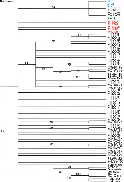
Two phylogenetic trees were constructed using parsimony and Bayesian analyses. In the parsimony tree (fig. 3) all the haplotypes present in East Scotland (blue) were clustered together along with the haplotypes SW2007/84 exclusive to the English Channel (orange) and the haplotype SW2006/98 which was present in Wales and the English Channel. Two haplotypes of the Mediterranean were also present in this cluster that is supported with a high bootstrap value (73). The Bayesian tree (Fig. 4) supports the same cluster with a very high posterior probability (91).

The exclusive haplotypes from the West Coast (red), one from the English Channel and one from Wales are all part of a polytomy with very low

bootstrap support (58) in the parsimony tree (fig. 3). In the Bayesian tree (fig. 4) four of the West Coast haplotypes, one of the English Channel and one of Wales were part of clusters that comprise sequences from Portugal,

(42)

[image:42.595.108.533.65.687.2]

Figure 3. Consensus Parsimony tree with 1000 bootstrap replicates. The outgroups were: Stenella spp, D. capensis, G. griseus, O. orca(2 haplotypes) andT. aduncus(2 haplotypes). Haplotypes from this study are shown in colors representing where they came from East Coast (blue), West Coast (red), Wales (green) and English Channel (pink).

(43)

[image:43.595.89.410.80.582.2]

Figure 4. Consensus Bayesian tree showing posterior probabilities. Two haplotypes of O. orca were used as an outgroup. Haplotypes from this study are shown in colors

representing where they came from East Coast (blue), West Coast (red), Wales (green) and English Channel (pink).

0.1 OorcaH13

Oorca Ggriseus_Schinensis

(44)

2.3.2. Microsatellites

2.3.2.1. Genetic diversity

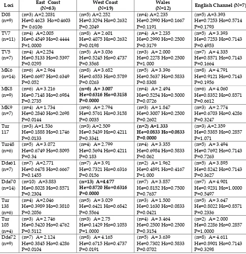
Of twenty microsatellites originally selected, 17 amplified successfully using multiplex conditions. Table 7 shows the percentage of error for each locus in both strandings and biopsies. Locus D22 shows over 20% of error for both biopsies and strandings. Loci TV5, MK9 and Dde84 show over 20% only for strandings but not for biopsies and locus Dde 70 shows over 20% only for biopsies. In LG1 a total of 10 biopsied individuals and 17 strandings were repeated representing 23.8% of total biopsies and 24.63 % of total strandings. In LG2 a total of 13 biopsied individuals and 30 strandings were repeated, representing 30.95% of the total biopsies and 43.47% of total strandings. Finally LG3 repeated 5 biopsied individuals that represent 11.9% of the total biopsies and 24 stranded individuals that represent 34.78 % of total

strandings. Locus Dde70 remained in the dataset because the sample size to calculate the error rate for biopsies in LG3 was only n=11 and due to the nature of the error rate scoring this values seems to be inflated.

The 17 loci were analysed in 110 individuals for linkage disequilibrium and three pairs resulted with highly significantp-valuesfor the test. These were (Tur61/Dde70), (D22/Dde84) and (Dde84 and Dde72). All the loci were also tested for Hardy-Weinberg deviations and if they were out of equilibrium after Bonferroni correction in more than one population (Table 8) they were eliminated from the analysis. Finally, Microchecker’s results show that Locus EV1 showed the presence of null alleles and an excess of heterozygotes.

(45)

data was analyzed with 13 loci. Details of genotype scoring process are shown in Appendix C.

Table 7. Genotyping error in biopsies and strandings. A total of 42 biopsies and 69 strandings were analyzed. In LG1 biopsies were repeated in average 2.6 times and strandings 2.5 times. In LG2 biopsies were repeated in average 2.46 times and strandings 2.7 times and LG3 repeated biopsies in average 2.2 times and strandings 2.5 times.

Locus Locus Group

Motif repeated

Error Biopsies

Error Strandings

D08 LG1 TG 0.05 0.1 D22 LG1 (CA)-TA-(CA) 0.24 0.297

TV7 LG1 CA 0.05 0.094

TV5 LG1 CA 0 0.222

MK6 LG1 GT 0 0.053

MK8 LG2 GT 0.088 0.049 EV1 LG2 (AC)(TC) 0.087 0.167

MK9 LG2 CA 0 0.225

Tur117 LG2 GATA 0 0.03 Tur91 LG2 GATA 0 0.15 Tur48 LG2 GATA 0 0.08 Dde61 LG3 CTAT 0.083 0.035 Dde70 LG3 CA 0.2727 0.155 Tur138 LG3 GATA 0.0909 0.019 Tur105 LG3 GATA 0 0

Dde84 LG3 CA 0 0.212

Dde72 LG3 CTAT 0.091 0.1

(46)

(MK8 and Dde70) and Wales (Tur117), for this reason they were kept in the analysis (Table 7).

Overall low heterozygosity values are present in all the populations except for the English Channel individuals that showed the highest values. Allelic

(47)

[image:47.595.87.587.165.682.2]

Table 8. Genetic diversity in nuclear microsatellites for all the populations. Sample size (N). For each locus: total number of alleles (n), Observed (Ho) and expected (He)

heterozygosity, number of alleles (n) and allelic richness (A). Loci out of equilibrium are shown in bold.

Loci East Coast_(N=63) West Coast_(N=19) _(N=12)Wales English Channel (N=7)

D08

(n=9) (n=3) A=2.2031He=0.4623 Ho=0.4603 P= 0.6106 (n=5) A=2.252 He=0.3294 Ho=0.2632 P=0.2049 (n=4) A=2.235 He=0.2990 Ho=0.1667 P=0.1191 (n=5) A=3.393 He=0.7253 Ho=0.5714 P=0.1793 TV7

(n=11) (n=4) A=2.005He=0.4549 Ho=0.4444 P=1.0000

(n=8) A= 2.601 He=0.4075 Ho=0.2632 P=0.0198

(n=4) A= 2.235 He=0.2990 Ho=0.2500 P=0.3179

(n=5) A= 3.393 He=0.7253 Ho=0.7143 P=0.4953

TV5

(n=7) (n=4) A=2.254He=0.5133 Ho=0.5397 P=0.0295

(n=5) A= 3.036 He=0.5245 Ho=0.4737 P=0.3568

(n=3) A= 2.000 He=0.2278 Ho=0.2500 P=1.000

(n=7) A= 4.335 He=0.8571 Ho=0.7143 P=0.1664

MK6

(n=14) (n=6) A= 2.964He=0.6697 Ho=0.6349 P=0.052

(n=8) A= 3.682 He=0.6553 Ho=0.5789 P=0.0263

(n=5) A= 3.396 He=0.5637 Ho=0.5833 P=0.8308

(n=8) A= 4.791 He=0.9121 Ho=0.7143 P=0.1956

MK8

(n=9) (n=6) A= 3.216He=0.7148 Ho=0.6984 P=0.2735

(n=6) A= 3.007 He=0.6316 Ho=0.3158 P=0.0000

(n=4) A= 2.494 He=0.5254 Ho=0.5000 P=0.0726

(n=6) A= 4.060 He=0.8352 Ho=0.8571 P=0.6612

MK9

(n=7) (n=4) A= 1.734He=0.2840 Ho=0.2698 P=0.0144

(n=6) A= 2.794 He=0.5761 Ho=0.3158 P=0.0035

(n=3) A= 1.847 He=0.3007 Ho=0.2500 P=0.2602

(n=3) A= 2.774 He=0.6703 Ho=0.4286 P=0.3247

Tur

117 (n=3) A=1.536He=0.1888 Ho=0.1746 P=0.0133 (n=3) A=2.509 He=0.5439 Ho=0.4211 P=0.3341 (n=2) A=1.333 He=0.0833 Ho=0.0833 P=0.0000 (n=3) A=2.359 He=0.5385 Ho=0.2857 P=1.071 Tur48

(n=6) (n=5) A= 3.072He=0.6749 Ho=0.8095 P=0.34

(n=4) A= 2.799 He=0.5694 Ho=0.4211 P=0.183

(n=4) A= 3.355 He=0.6984 Ho=0.5833 P=0.062

(n=5) A= 3.494 He=0.7692 Ho=0.7143 P=0.7263

Dde61

(n=7) (n=7) A=2.771He=0.6478 Ho=0.6667 P=0.1455

(n=7) A= 3.91

He=0.7321 Ho=0.6316 P=0.0156

(n=2) A= 1.962 He=0.4891 Ho=0.4167 P=1.000

(n=5) A= 3.895 He=0.8242 Ho=0.7143 P=0.3627

Dde70

(n=14) (n=10) A=3.883He=0.8028 Ho=0.8571 P=0.2304

(n=13) A=4.477 He=0.8720 Ho=0.6316 P=0.0000

(n=7) A= 3.857 He=0.8152 Ho=0.7500 P=0.7637

(n=7) A= 4.901 He=0.9231 Ho=1.0000 P=0.5497 Tur 138 (n=6) (n=4) A=2.046 He=0.3989 Ho=0.3810 P=0.2056

(n=5) A= 3.029 He=0.6421 Ho=0.6842 P=0.5564

(n=3) A= 1.500 He=0.1630 Ho=0.0833 P=0.0421

(n=5) A= 3.647 He=0.8022 Ho=0.8571 P=0.2336

Tur 105 (n=4)

(n=3) A= 2.746 He=0.5420 Ho=0.4762 P=0.5112

(n=3) A= 2.75

He=0.1429 Ho=0.1053 P=1.0000

(n=4) A= 3.464 He=0.2500 Ho=0.2500 P=0.3154

(n=2) A= 2.000 He=0.2286 Ho=0.2857 P=1.0000

Dde72

(n=9) (n=7) A= 2.124He=0.3845 Ho=0.4286 P=0.0104

(n=8) A= 4.165 He=0.6715 Ho=0.4737 P=0.0191

(n=5) A= 3.639 He=0.7302 Ho=0.5833 P=0.0702

(48)

2.3.2.2. Population Structure: Three different methods to estimate Population differentiation

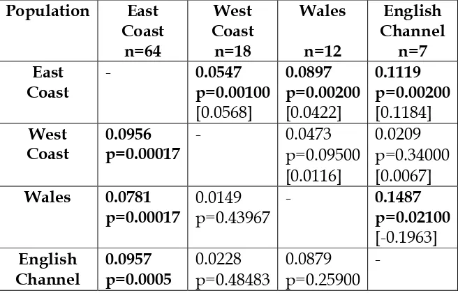
Pairwise population differentiation indicesFST, RhoSTand DESTwere calculated for all populations (Table 8). Significant values were in all

[image:48.595.86.414.364.574.2]

comparisons of the East Coast with other locations. Population differentiation was stronger between the East Coast of Scotland and the English Channel. Other pairwise comparisons were not significant, possibly due to the reduced sample sizes of these populations compared to the East Coast.

Table 8. Population differentiation between pairwise populations with microsatellites. Significant scores are in bold and the p-value is shown below them. Lower diagonal shows Fstvalues (P-valueswere obtained after 6000 permutations). Average variance components ofRhoSTshown in the upper diagonal along with Jost’s (2008)DEST shown in [].

2.3.2.2. Bayesian clustering assignment of populations (The problem of determining K)

Structure was run with the number of populations set from 1 to 10. Evanno et al. (2005) recommendations were followed using the admixture model with correlated frequencies among populations. This model is recommended when populations are likely to have a common ancestor.

Population East Coast n=64 West Coast n=18 Wales n=12 English Channel n=7 East Coast -0.0547 p=0.00100 [0.0568] 0.0897 p=0.00200 [0.0422] 0.1119 p=0.00200 [0.1184] West Coast 0.0956

p=0.00017 - 0.0473p=0.09500 [0.0116]

0.0209 p=0.34000 [0.0067]

Wales 0.0781

p=0.00017 0.0149p=0.43967

-0.1487 p=0.02100 [-0.1963] English Channel 0.0957

p=0.0005 0.0228p=0.48483

0.0879 p=0.25900

(49)

-In fig. 5 the average value of LnP(D) for each value of K simulated was plotted. The results show a plateau, but it is not clear whether the plateau starts at K=3 or K=4. The difference in the average of the log-likelihood values between K=3 and K=4 is around 30. Pritchard et al.(2007) suggests that when the differences are so small, the true value of K is more likely to be the smaller of the two.

Average of Ln P(D) with admixture model

-3550 -3500 -3450 -3400 -3350 -3300 -3250 -3200 -3150 -3100 -3050

0 1 2 3 4 5 6 7 8

K A v e ra g e L n P (D )

Figure 5. Average value of the LnP(D) of the posterior probability for ten runs of each K for

Admixture Model.

Following the Evanno et al. (2005) procedure for deciding the true value of K, I calculated the rate of change between the different values of K. This detects the value of K for the uppermost level population structure for the

populations tested (fig. 6). This method identifies K=2 as the number of subgroups.

Determination of K with admixture model

0 20 40 60 80 100 120 140

1 2 3 4 5 6 7

K D e lt a K

Figure 6. Graphical representation of ΔK calculated as: ΔK= ׀L’’(K)׀/SD[L(K]. This graph is

(50)

The ‘No admixture model’ was also tested with our data. Structure

recommends this model for populations that are fully discrete and it is meant to be better at detecting subtle structure. This model assumes that all the individuals come from just one population. The average LnP(D) for the posterior probabilities is shown in fig. The start of the plateau is not clear either K=3 or K=4.

Average LnP(D) for each K with No Admixture Model -3600 -3500 -3400 -3300 -3200 -3100 -3000

0 2 4 6 8 10 12

K A v e ra g e L n P (D )

Figure 7. Average value of the Ln of the posterior probability for ten runs of each K for ‘No

admixture model’.

The Evanno et al. (2005) procedure again identified the maximum value of K

at K=2 and we can observe another peak of ΔK at K=4 but much lower.

Determination of K from No-admixture model

0 100 200 300 400 500 600

0 2 4 6 8 10

K D e lt a K

Figure 8. Graphical representation of ΔK calculated as: ΔK= ׀L’’(K)׀/SD[L(K]. This graph is the

(51)

These results give us 2 different scenarios. K=4 implies the East Coast of Scotland is isolated from the rest of the neighbouring populations, which is consistent with theFstresults. A connection between a part of the West Coast of Scotland that includes the Barra biopsied individuals is connected with Wales. The other part of the West Coast is clustered with the English Channel animals (fig. 9).

Figure 9. Barplot of the likelihood (Y-axis) of each individual’s (X-axis) assignment to a particular population for K=4. Pop 1= East Coast of Scotland (Moray Firth), Pop 2= East Coast of Scotland Outer Community, 3) West Coast of Scotland, Pop 4= Wales and Pop 5= English Channel.

When the Evanno et al. (2005) procedure is applied we obtain K=2 and the scenario suggests a connection between the East Coast of Scotland, part of the West Coast of Scotland and most of Wales. On the other hand the rest of the West Coast of Scotland and England (fig. 10).

Figure 10. Barplot of the likelihood (Y-axis) of each individual’s (X-axis) assignment to a particular population for K=2. Pop 1= East Coast of Scotland (Moray Firth), Pop 2= East Coast of Scotland Outer Community, 3) West Coast of Scotland, Pop 4= Wales and Pop 5=

Moray Firth Outer Moray Firth Barra West

Coast Wales England Moray Firth Outer Moray Firth Barra

West

(52)

The scenario with K=3 maintains a deep division in the West Coast of Scotland into 2 groups, Barra and the rest of the West Coast. The Barra individuals grouped with Wales while the rest of the West Coast has a connection with the population from English Channel. In this scenario the East Coast of Scotland is not isolated and a proportion of individuals belong to the same cluster as the Barra-Wales individuals.

The main problem with the different K’s is the establishment of gene flow between the East Coast of Scotland, Wales and Barra. It is clear in all the possible outcomes of K, that there is a connection between the West Coast of Scotland population of Barra and Wales. The individuals from the English Channel and the rest of the West Coast of Scotland are also consistent throughout all the scenarios.

Figure 11. Barplot of the likelihood (Y-axis) of each individual’s (X-axis) assignment to a particular population for K=3. Pop 1= East Coast of Scotland (Moray Firth), Pop 2= East Coast of Scotland Outer Community, 3) West Coast of Scotland, Pop 4= Wales and Pop 5= English Channel

Results for only the East Coast samples with the admixture model do not include the Evanno method as it fails to acknowledge only one population. The average of the LnP (D) for each K is shown in fig. 12. The best values are for K=2 and K=3, with very similar likelihoods, -1540.8 and -1539.6

respectively.

Moray Firth Outer Moray Firth Barra West

(53)

Average Ln P (D) with admixture model for the East Scottish population

-1700 -1650 -1600 -1550 -1500

1 2 3 4 5 6 7 8 9 10

K

A

v

e

ra

g

e

L

n

P

(D

)

Figure 12. Average value of the LnP(D) of the posterior probability for eight runs of each K for

Admixture Model.

For K=2 the analyzed individuals have almost a 50% probability to belong to either of the 2 populations (Table 9). When K=3 the probabilities for each inferred cluster are even lower. The barplots in fig. 13 show the graphic representation for both scenarios K=2 and K=3 where there is no obvious distinction between strandings and biopsies. The only safe conclusion is that the samples come from one population.

Table 9. The probabilities of assigning individuals to a particular population given a particular value of K

Given K

Inferred Clusters No of Individuals

2 1 2

0.470 0.530

63

3 1 2 3

0.381 0.357 0.263

(54)

Figure 13. Barplots of the East Scottish population. The upper barplot represents to K=2 and the lower barplot to K=3. The biopsied individuals are shown within the black lines and the last 4 individuals are also strandings.

2.3.2.3. Determination of migration rates and sex-biased dispersal

To clarify the ambiguity in determining the true value of K, the mean

migration rates along with 95% confidence intervals were calculated with the program BayesAss 1.3 (Table 11). This program calculates the proportion of individuals that do not migrate, described as the migration rate into the same population (diagonal shown in bold). It also calculates the migration rates from each population into another.

BayesAss 1.3 simulates migration rates and the correspondent confidence intervals for a dataset with no information on migration. This procedure gives us a mean migration rate and a confidence interval of values that are expected merely by chance. The migration rates obtained with the real data should be different to the rates and confidence intervals simulated with the same number of populations. In a scenario with 4 populations the mean migration rate for non migrants (diagonal) in a non informative data set is