Applied Mathematics, 2010, 1, 37-43
doi:10.4236/am.2010.11006 Published Online May 2010 (http://www.SciRP.org/journal/am)
Implied Bond and Derivative Prices Based on Non-Linear
Stochastic Interest Rate Models
Ghulam Sorwar
1, Sharif Mozumder
21Nottingham University Business School, Jubilee Campus, Nottingham, UK 2Department of Mathematics, University of Dhaka, Dhaka, Bangladesh E-mail: [email protected], sharif_math2000@yahoo.com
Received March 8, 2010; revised April 2, 2010; accepted April 30, 2010
Abstract
In this paper we expand the Box Method of Sorwar
et al.
(2007) to value both default free bonds and interest
rate contingent claims based on one factor non-linear interest rate models. Further we propose a one-factor
non-linear interest rate model that incorporates features suggested by recent research. An example shows the
extended Box Method works well in practice
.Keywords:
Stochastic, Interest Rates, Derivatives, Box Method
1. Introduction
Stochastic differential equations are the foundations on which modern option pricing methodology is based. However, non-linear stochastic differential equations for interest rate models have been proposed that captures the non-linear dynamics of the spot interest rates. There are two aspects to the modeling of interest rate term structure models and interest rate contingent claims. The first concerns the econometric aspects (see for example, [1]) and the second the numerical implementation of the re-sulting models. With regard to the numerical aspects of interest rate modeling, there exist three different ap-proaches. The first is the lattice approach introduced by Cox-Ross-Rubinstein (1979) [2]. However, as Ba-rone-Adesi, Dinenis and Sorwar (1997) [3] have demon-strated the lattice approach does not always lead to mea-ningful bond and hence contingent claim prices. The second approach is the Monte-Carlo simulation approach introduced by Boyle (1977) is mainly used to value path dependent European type contingent claims. To date no single accepted Monte-Carlo simulation scheme has been put forward for the valuation of American type contin-gent claims. The third approach is the partial differential equation (PDE) approach. With this approach, the par-tial first and second order derivatives are discretized to produce a system of equations which are then solved iteratively to obtain the bond and contingent claim prices. However, Sorwar et al. (2007) have shown that the usual finite difference approach used to discretize the PDE does not always lead to bond and contingent claim prices
that correspond with analytical prices where these prices are available.
Sorwar et al. (2007) introduced the Box Method from engineering to improve on the standard finite difference approach. Sorwar et al. (2007) focused on the CKLS (1992) model. Sorwar et al. (2007) did not attempt to value bonds and contingent claims based on non-linear interest rate models. Ait-Sahalia (1996) [4] non-and Conley et al. (1997) [5] propose parametric linear one-factor which allows non-linear parameterisation. Our main objective in this paper is to expand the Box Method of Sorwar et al. (1997) to price bonds and contingent claims based on both linear and non-linear interest rate models.
The outline of the paper is as follows: Section 2 the general non-linear parametric model and the resulting partial differential equation for default free bonds and contingent claims is outlined. We then derive the Ex-panded Box Method (EBM) for the valuation of default free bonds and contingent claims. Using US estimates we compute implied bond and contingent claims prices in Section 3. Section 4 contains a summary and conclusion.
2. Expanded Box Method (EBM)
In this section we discuss the valuation of the bond and contingent claim prices based on the extended Ait-Sahalia (1996) [4] and Conley et al. (1997) [5] framework. Following Sorwar et al. (2007) we let:
(
*)
t
Table1. lternative Parametric Specifications of the Spot Interest Rate Process
( )
2( )
t t t t
dr =µ r dt+σ r dW . Drift function
( )r
µ Diffusion function σ2( )r
Reference
0 1r
α +α β0 Vasicek (1977) [6]
0 1r
α +α β1r Cox-Ingersoll-Ross(1985) [7]
Brown-Dybvig(1986) [8] Gibbons-Ramaswamy(1993) [9]
0 1r
α +α 2
2r
β Courtadon (1982) [10]
0 1r
α +α 3
2rβ
β Chen et al. (1992)
2 3 0 1r 2r αr
α +α +α + β0+β1r+β2rβ3 Ait-Sahalia (1996) [4]
3 5 4 0 1r 2r
r
α α
α
α +α +α + β0+β1r+β2rβ3
matures at time T* with the generated spot rate
t
r .
(
*)
P t,T ,T : price of a contingent claim at time
t
which expires at time T based on a discount bond which matures at time T* subject to suitable boundaryconditions.
In a risk-neutral world, the drift rate is adjusted by the market price of risk λr1 so that the short-term interest
process becomes:
(
)
(
3 5)
3
0 1 2 4
0 1 2
t
t
dr r r r dt
r r dW
α α
β
α α λ α α
β β β
−
= + + + + +
+ + (1)
The resulting partial differential equation is:
(
)
33 5
2
0 1 2 2
0 1 2 4
1 2
0
U
r r
r
U U
r r r rU
r t
β
α α
∂
β β β
∂
∂ ∂
α α λ α α
∂ ∂
−
+ +
+ + + + + − + =
(2) In equation (2) U r ,t
( )
t may represent either(
*)
t
B r ,t,T or P t,T ,T
(
*)
subject to the appropriateboundary conditions (see [10] for more details). Follow-ing Sorwar et al. (2007) we transform the above pricing equation such that either the bond or the contingent claims evolves from the options expiration date or the bonds maturity date to the present, i.e. we let τ = −T t.
The above equation then becomes:
(
)
3 53 2
0 1 2 4
2
0 1 2
2 r r r
U U
r
r r r
α α
β
α α λ α α
∂ ∂
∂
∂ β β β
−
+ + + +
+ −
+ +
3 3
0 1 2 0 1 2
2r U 2 U
r rβ r rβ ∂
∂τ
β +β +β = β +β +β (3)
We now choose a general function R r, ,
(
α β)
such that:(
)
3 53 2
2
0 1 2 4
0 1 2
1
2
U U
R
R r r r
r r r U
r r r
α α
β
∂ ∂ ∂
∂ ∂ ∂
α α λ α α ∂
∂
β β β
−
= +
+ + + +
+ +
(4)
The above expression simplifies to yield:
(
)
3 53
0 1 2 4
0 1 2
1 R 2 r r r
R r r r
α α
β
α α λ α α
∂
∂ β β β
−
+ + + +
=
+ +
(5)
We now integrate from the general value
r
(
rn−1< <r rn+1)
to the lower limit of integration r=0to obtain:
(
)
(
)
3 53 1
0 1 2 4
0 1 2
2
n
r
r
R r, ,
r r r
exp dr
r r
α α
β α β
α α λ α α
φ
β β β
−
− =
+ + + +
+
+ +
∫
where φ=ln R , ,
(
0α β)
. We further note that:1 R U 1 Q U
R r r Q r r
∂ ∂ ∂ ∂
∂ ∂ ∂ ∂
=
where: 1Risk premium is treated differently by researchers. Vasicek (1977) [6]
G. SORWAR ET AL. 39
(
)
(
)
3 53
0 1 2 4
0 0 1 2
2r
Q r, ,
r r r
exp dr
r r
α α
β α β
α α λ α α
β β β
− =
+ + + +
+ +
∫
So equation (3) becomes:
3
0 1 2
1 Q U 2r U
Q r r r rβ
∂ ∂
∂ ∂ β β β
− =
+ +
We now transform the interest rate as:
3
0 1 2
2 U
r rβ
∂ ∂τ β +β +β
(6)
cr
cr
s
+
=
1
where c is a constant. (7)This leads to the transformation of equation (6) as:
( )
( )
(
)
(
)
(
)
(
)
(
)
(
)
3 3
3 2
2
1 1
0 2 0 2
1 2 2 1
1 1
1 1 1 1
U s U U
s
Q s s s c s s s c s s s
c s c s c s c s
β β τ
β β
β β β β
∂ Ψ ∂ − = ∂
∂ ∂ − − ∂
+ + + +
− − − −
(8)
where:
( ) (
) ( )
( )
(
)
(
)
(
)
(
)
(
)
(
)
(
)
3 5
3 2
1
0 2 4
2
0 1
0 2
1
1 1 1
2 1
1 1
s
s c s Q s
s s s
c s c s c s
Q s exp dr
c s s s
c s c s
α α
β α λ
α α α
β
β β
−
Ψ = −
+
+ + +
− − −
=
−
+ +
− −
∫
Following the set-up of Sorwar et al. (2007) a grid of size M N× is constructed for values of
(
)
m n
U =U n r,m t∆ ∆ - the value of U at time increment
m
t and interest rate increment sn, for each method,
where:
0
m
t = + ∆t m t m=0 1, ,....,M 2
1
n n
s+ s a
∆ = ∆ + n=1,....,N
where a is an arbitrary constant.
Using the Euler backward difference for the time de-
rivative gives: U U U0
t ∂
∂τ − =
∆ ,
where U0 and Urefers to bond or contingent claims
prices at time step m-1 and m respectively. Integrating equation (8) from the point
1 1
2
2
n n
n
s
s
s
−−
+
=
to point 11
2
2
n n
n
s
s
s
++
+
=
, we have:( )
(
)
( ) ( )
(
)
( ) ( )
(
)
( ) ( )
1 1 1
2 2 2
1 1 1
2 2 2
1 2
1 2
3 2
2
0 2
1
2 2
1 1
1 2
1
n n n
n n n
n
n
s s s
s s s
s
s
U s
t s ds t Q s f s Uds Q s f s Uds
s s c s c s
Q s f s U ds
c s
+ + +
− − −
+
−
∂ ∂
−∆ Ψ + ∆ +
∂ ∂ − −
=
−
∫
∫
∫
∫
(9)
Discretizing each of the above integrals, and rearrang-ing gives us the followrearrang-ing matrix equation:
1
1 1
m m m m
n nU n nU n nU n nU
α − χ η β
− +
= + + (10)
where:
( )
12
1 2
n
n
s
s
U
t s ds
s s
+
−
∂ ∂
−∆ Ψ +
∂ ∂
∫
(
)
( ) ( )
12
1 2
3 2
2
1
n
n
s
s
s
t Q s f s Uds c s
+
−
∆ +
−
∫
2Where a and
0 s
(
)
( ) ( )
1 2 1 2 2 1 2 1 n n s sQ s f s Uds c s + − −
∫
(
)
( ) ( )
1 2 1 2 0 2 1 2 1 n n s sQ s f s U ds c s
+
−
=
−
∫
(9)Discretizing each of the above integrals, and rearrang-ing gives us the followrearrang-ing matrix equation:
1
1 1
m m m m
n nU n nU n nU n nU
α − χ η β
− +
= + + (10)
where:
( )
( )
( )
( )
( )
( )
( )
( )
( )
(
)
(
)
( )
(
)
(
)
1 2 1 2 1 1 2 2 1 1 2 2 1 1 2 2 1 1 1 0 1 1 10 2 3
1 2 2 2 2 1 1 n n n
n n n
n n
n n n
n n
n
n n n n n n
n n n n n n n n n I s t
s s Q s
s t
s s Q s
s s
t t tI I
s s Q s s s Q s
s f s
I s s
c s
f s
I s s
c s α χ β η − − + + − + − + + − + − = Ψ −∆ = − Ψ −∆ = − Ψ Ψ ∆ ∆ = + + ∆ + − − = − − = − −
The matrix equation linking all bond prices or contingent claim prices between two successive time steps m-1 and
m is:
1 0 1
1 0 1
1
1 1 0 1
2 2 2 0 1
3 3 3
3 3 3
2 2 2
1 1 1
0 0 0 0
0 0 0
0 0 0
0
0 0
0 0 0
m m m N N m m
N N N
N N N
m
N N N N
U U U U U U α α α
η β α
χ η β α
χ η β
χ χ β
χ η β
χ η α
− − − − − − − − − − − − =
Sorwar et al. [12] used the following SOR iteration process to determine bond and contingent claims prices:
(
1 1)
1 1
1
m m m m
n n n n n n n
n
z αU χU βU
η − − +−
= − − (11)
In particular they evaluated bond using the following expression:
(
1)
1m m m
n n n
U =ωz + −ω U − (12)
Contingent claims were calculated using:
(
1)
1m m m
n n n
U =max Z , z ω + −ω U −
(13)
where Z is the intrinsic value of the contingent claim and for n=1,...,N-1, and ω ∈
(
1 2,]
3.3. Analysis of Results
In this section we apply the EBM using recent estimates of the non-linear model of Ait-Sahalia (1996) [4] on 7-day Eurodollar deposit spot rate over 1973-1995 to demonstrate the method. Ait-Sahalia (1996, Table 4) [4] obtained the following estimates:
3
0 1
2 1
2 3
4 643 10
4 333 10 1 143 10 2
. , . , . , , α α α α − − − = − × = × = − × = 4 4 1 304 10. , 5 1
α = × − α = .
4
0 1
3 3
2 3
1 108 10
1 883 10 9 681 10 2 073
[image:4.595.55.279.484.690.2]. , . , . , . β β β β − − − = × = − × = × = .
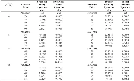
Table 2 reports the bond prices for maturities ranging from 6 months to 30 years and across interest rates of 2% to 16%. Table III reports both the value of call and put options across a wide range of interest rates. We consider both short and long dated call and put options. The short dated call and put options are based on a 5-year bond with an expiry date of 1 year and is during the last year before the bond matures. Similarly long dated options are based on 10-year bond with an expiry date of 5 years during the last 5 years of the bond. Finally both call and put option prices are calculated across a wide range of exercise prices. The exercise prices are chosen so as to highlight variation of prices for both in-the-money and out-of-the-money options. We assume λ, the market price of risk is zero.
Turning to Table 2, we find that at lower interest rate bond prices decay slowly as the term to maturity in-creases. For example, at 2% interest rate a 1 year matur-ity bond is valued at 98.1119, whilst a 30 year bond is valued at 74.8290. At high interest rates, the bond price decay is more rapid for example at 16% interest rate, a 1 year maturity bond is valued at 85.2915, whist a 30 year maturity bond is valued at 1.1770. Turning to Table 3, we observe the following features. Short expiry call op
3ω is determined by numerical experimentation. For all our
G. SORWAR ET AL. 41
Table 2. All options written on zero coupon bonds with a face value of $100.00.
Interest Rate Maturity
of Bond 2% 4% 6% 8% 10% 12% 14% 16%
0.5 99.0286 98.0370 96.9855 96.0885 95.1315 94.1844 93.2506 92.3403
1 98.1119 96.1434 94.0805 92.3406 90.5050 88.7059 86.9566 85.2915
5 92.2400 83.3035 74.3413 67.4685 60.8623 54.9010 49.7324 45.6212
10 87.0431 71.9535 56.7017 46.1717 37.2750 30.1193 24.7834 21.3038
15 83.1089 64.1538 44.6651 32.1800 22.9491 16.5267 12.3933 10.1317
20 79.9228 58.6473 36.4723 22.9644 14.3178 9.0809 6.2237 4.8889
25 77.2156 54.6338 30.8731 16.8832 9.0110 5.0032 3.1400 2.3870
30 74.8290 51.6021 27.0075 12.8582 5.7491 2.7679 1.5921 1.1770
Table 3. All options written on zero coupon bonds with a face value of $100.00.
r
(%)
Exercise-Price5 year ma-turity 1 year
ex-piry
5 year ma-turity 1 year
ex-piry
Exercise-Price
10 year maturity 5 year ex-piry
10 year maturity 5 year ex-piry
(83.3035) call put (71.9535) call put
4 70 16.0031 0.0000 60 21.9713 0.0007
75 11.1959 0.0000 65 17.8062 0.0493
80 6.3895 0.0050 70 13.6418 0.6489
85 1.9369 1.6966 75 9.5270 3.1894
90 0.1421 6.6966 80 5.7979 8.0466
(67.4685) (46.1717)
8 55 16.6811 0.0000 35 22.5578 0.0000
60 12.0641 0.0000 40 19.1843 0.0000
65 7.4471 0.0000 45 15.8109 0.0058
70 2.8302 2.5315 50 12.4375 3.8283
75 0.0203 7.5315 55 9.0641 8.8283
12 (54.9010) (30.1193)
45 14.9341 0.0000 20 19.1395 0.0000
50 10.4996 0.0000 25 16.3942 0.0000
55 6.0652 0.1561 30 13.6492 0.0183
60 1.6310 5.1561 35 10.9042 4.8804
65 0.0000 10.1561 40 8.1591 9.8804
16 (45.6212) (21.3038)
35 15.7692 0.0000 10 16.7416 0.0000
40 11.5046 0.0000 15 14.4606 0.0000
45 7.2400 0.0005 20 12.1795 0.0001
50 2.9755 4.3788 25 9.8985 3.6962
55 0.0129 9.3782 30 7.6174 8.6962
tions decay faster than longer expiry call options; for example at r = 4%; the price of a call option decreases from 16.0031 to 11.1959 when the exercise price in creases from 70 to 75. For a similar 5 year call option the price decreases from 21.9713 to 17.8062, when the exer-cise price increases from 60 to 65. Furthermore, the call option prices decrease at a slower rate at high interests. This feature becomes more pronounced for longer expiry call options. With regard to put options we find, the prices are very close to zero, when the options are at-the- money or out-of-the-money. Finally, we find that the value of in-the-money put options is dominated by the
intrinsic-value.
4. Conclusions
[image:5.595.74.520.306.577.2]Expanded Box Method works well with the example considered.
5. References
[1] K. C. Chan, G. A. Karolyi, F. A. Longstaff and A. B. Sanders, “An Empirical Comparison of Alternative Mod-els of the Short-Term Interest Rate,” Journal of Finance, Vol. 47, No. 3, 1992, pp. 1209-1227.
[2] J. C. Cox and S. A. Ross, “Option Pricing: A Simplified Approach,” Journal of Financial Economics, Vol. 7, No.
3, 1979, pp.229-264.
[3] G. Barone-Adesi, E. Dinenis and G. Sorwar, “A Note on the Convergence of Binomial Approximations for Interest Rate Models,” Journal of Financial Engineering, Vol. 6, No. 1, 1997, pp. 71-78.
[4] Y. Ait-Sahalia and Y. Testing “Continuous-Time Models of the Spot Interest Rate,” Review of Financial Studies, Vol. 9, No. 2, 1996, pp. 385-426.
[5] T. G. Conley, L. P. Hansen, E. G. J. Luttmer and J. A. Scheinkman, “Short-Term Interest Rates as Subordinated Diffusions,” Review of Financial Studies,Vol. 10, No. 3, 1997, pp. 525-577.
[6] O. A. Vasicek, “An Equilibrium Characterization of the Term Structure,” Journal of Financial Economics, Vol. 5, No. 2, 1977, pp. 177-188.
[7] J. C. Cox, J. E. Ingersoll and S. A. Ross, “A Theory of the Term Structure of interest Rates,” Econometrica, Vol. 53, No. 2, 1985, pp. 385-407.
[8] S. J. Brown, P. H. Dybvig, “The Empirical Implications of the Cox, Ingersoll, Ross Theory of the Term Structure of Interest Rates,” Journal of Finance, Vol. 41, No. 3, 1986, pp. 617-630.
[9] M. R. Gibbons and K. Ramaswamy, “A Test of the Cox, In-gersoll, and Ross Model of the Term Structure,” Review of Financial Studies, Vol. 6, No. 3, 1993, pp. 619-658.
[10] G. Courtadon, “The Pricing of Options on Default-Free Bonds,” Journal of Financial and Quantitative Analysis, Vol. 17, No. 1, 1982, pp. 75-100.
[11] A. Settari and K. Aziz, “Use of Irregular grid in Reservoir Simulation,” Society of Petroleum Engineering Journal, Vol. 12, No. 2,1972, pp. 103-114.
G. SORWAR ET AL. 43
Appendix
( )
( )
( )
1 2
1 1
2 2
1 1
1
2 2
2
n
n n
n
s
n n
s s
s
U U U
s ds s s
s s s s
+
+ −
−
+ −
∂ Ψ ∂ ≈ Ψ ∂ − Ψ ∂
∂ ∂ ∂ ∂
∫
Further:
1 2
1 2
1 1
1 1
n
n
m m
n n
s n n
m m
n n
s n n
U U U
s s s
U U U
s s s
+
−
+
+
−
− − ∂
≈
∂ −
− ∂
≈
∂ −
Substitution of the above approximation yields:
( )
( )
( ) ( )
( )
1
2 1
2
1 2
1 1 1
2 2 2
1 1
1
1 1 1
n
n
s
n m
n
n n
s
n n m n m
n n
n n n n n n
s U
s ds U
s s s s
s s s
U U
s s s s s s
+
−
+ + +
+ − −
−
+ − −
Ψ
∂ Ψ ∂ ≈ −
∂ ∂ −
Ψ Ψ Ψ
+ +
− − −
∫
(
)
( ) ( )
12
1 2
3 2
2
1
n
n
s
s s
t f s Q s Uds
c s
+
−
∆ ≈
−
∫
( )
(
)
( )
12
1 2
3 2
2
1
n
n
s m n n s
s
tQ s U f s ds
c s
+
− ∆
−
∫
We further take:
(
)
( )
(
)
( )
(
)
12
1 1
2 2
1 2
3 3
2 1 2 1
n
n
s
n
n n n
s n
s
s f s ds f s s s
c s c s
+
−
+ −
≈ −
− −
∫
Similar approximation yields:
(
)
( ) ( )
( )
(
)
( )
(
)
(
)
( ) ( )
( )
(
)
( )
(
)
12
1 2
1 1
2 2
1 2
1 2
1 1
2 2
2
2
0 2
1
2
1 2
1
1 2
1 1 2
1
1 2
1
n
n
n
n
s
s
m
n n n n n
n s
s
m
n n n n n
n f s Q s Uds
c s
Q s U f s s s
c s
f s Q s U ds
c s
Q s U f s s s
c s
+
−
+
−
+ −
−
+ −
≈ −
− −
≈ −
− −