The effects of public spending composition on firm productivity

The E¤ects of Public Spending Composition

on Firm Productivity

Richard Kneller

and Florian Misch

a_{School of Economics, University of Nottingham, Nottingham NG7 2RD, UK}

b_{Centre for European Economic Research, 68161 Mannheim, Germany}

February 21, 2014

Abstract

This paper exploits the unique institutional features of South Africa to estimate the impact of provincial public spending on …rm produc-tivity. In contrast to existing microeconomic evidence, we explore the e¤ects of …scal expenditures and remove the e¤ects of revenue rais-ing policies. Our identi…cation strategy is based on di¤erences in the e¤ects of public spending across …rms within the same industry and province. We show that public spending composition a¤ects produc-tivity depending on the capital intensity of …rms, with less capital intensive …rms being particularly a¤ected. These e¤ects appear to be robust.

JEL code: D24, H32, H72

Keywords: Public Spending Composition; Productive Pub-lic Spending; Firm Productivity

Generous …nancial support from Forfás is gratefully acknowledged. We thank the participants at a seminar in Dublin organized by Forfás for valuable comments. We are also grateful to Neil Rankin, the National Treasury, Republic of South Africa, and Kenneth Creamer who all faciliated the access and the use of the data used in this paper.

y_{Corresponding author. E-mail address: misch@zew.de / Telephone: +49 (0) 621 1235}

1

Introduction

It has long been understood within theories of economic growth and devel-opment that changes to …scal policy, including changes in the composition of public spending, a¤ect aggregate outcomes such as the rate of economic growth (Barro, 1990; Devarajan et al. 1996). Increasingly, cross-country em-pirical evidence has been found to support these model predictions. Adam and Bevan (2005), López and Miller (2007), and Hong and Ahmed (2009) all …nd for example, that greater productive expenditures, usually de…ned as in-cluding spending on transport, communication, education, and health, have signi…cant positive growth e¤ects (Gemmell et al., 2012, provide a recent survey).

The consistency of these …ndings suggests that they are robust. But be-cause they are generated using macro data, they are still subject to criticism of Schwellnus and Arnold (2008) that they hide variation in their e¤ects across …rms and leave unclear the mechanism through which they are e¤ec-tive. Complementary evidence at the micro level is relatively uncommon and focused on a relatively narrow set of questions however; an outcome of lim-ited availability of …scal expenditure data measured at a sub-national level. As a consequence the literature has concentrated on the e¤ects of changes to transport infrastructure, see for example Datta (2012), Shirley and Winston (2004) and Reinikka and Svensson (2002), and Arnold et al. (2008), or the investment climate more generally, see for example Bastos and Nasir (2004) and Dollar et al. (2005).1

In this paper we contribute to our understanding of the e¤ects of …scal policy by studying the e¤ect of changes to the mix of public spending on the productivity of South African …rms. For this task we exploit the richness of the …scal data for South Africa, which include detailed types of health, education and transport expenditures at the province level. In this regard we build most closely on the work of Bekes and Murakozy (2005) and Gabe (2003), who …nd somewhat mixed evidence for the e¤ects of …scal policy on …rms. Bekes and Murakozy (2005) …nd that in Hungary public investment by the central government had positive and signi…cant e¤ects on …rm

productiv-1_{Our paper is also related to a large literature that dates however at least back to}

ity, but that the e¤ect of public investment by municipalities was negative. Gabe (2003) uses expenditure and revenue data to explain the growth of U.S. …rms (measured as the change of employment), but …nds no signi…cant e¤ect from either.

Alongside our interest in the e¤ects of the mix of government spending we di¤er from the existing literature in our ability to disentangle this from revenue raising policies. At the provincial level in South Africa discretionary …scal policy exists for the mix of expenditures. All broad based taxes are identical across provinces, and borrowing at the sub-national level is limited.2

As a result, the level of public spending can be viewed as exogenous to the individual province as it is dependent on grants from the central government. This is important in light of …ndings from macro growth regressions which show that the implicit assumptions about how …scal changes are …nanced have a strong e¤ect on the relationship with growth (Kneller et al., 1999).

To preview our results, we …nd that reallocating public resources can af-fect the productivity of some …rms in the short to medium run (our data do not allow us to describe longer term impacts), where we use the capital-labor ratio to di¤erentiate di¤erent types of …rms. In this regard our …ndings support the argument of Schwellnus and Arnold (2008) that the e¤ects of …s-cal policy di¤er across …rms, and, in addition, demonstrate that one of the transmission mechanisms through which aggregate growth changes occur is by changes to the productivity of …rms. In our most parsimonious speci…ca-tions we …nd that increasing expenditures on education, health, and trans-port as a share of total expenditures has a robust, positive and signi…cant e¤ect on the productivity of …rms with the lowest capital-labor ratios (the bottom quartile).3 _{For those …rms that use capital-to-labor with a greater}

intensity the e¤ects are less frequently signi…cant, while for those …rms with the highest capital-labor ratios we …nd no e¤ect.

We test the robustness of our …ndings to the inclusion of a wide set of province-industry and time dummies that might plausibly capture the e¤ects of any omitted variables. For example, the productivity of …rms and the choice of province-level …scal expenditures might be a¤ected by time-invariant province-industry speci…c factors such as geography or climate. Or public expenditures might be targeted at particular industries in particular provinces because they have lower or higher productivity than elsewhere. Or it could occur that unobserved province-speci…c shocks a¤ect the productivity of …rms within a province and, through the automatic stabilizer mechanism,

2_{We describe the details of the system of …scal decentralization in the Appendix.} 3_{To correct for province-speci…c industry factors that cause the average capital-labor}

may generate a change to the mix of expenditures. We continue to …nd throughout this part of the paper evidence that …rms with di¤erent capital-labor ratios are a¤ected di¤erently by changes to the expenditure mix. We cautiously describe this evidence as indicating rising (short-run) productivity of those …rms with relatively low capital-labor ratios, and as consistent at least with a causal interpretation. The disadvantage of such an approach is that we cannot identify the overall magnitude of the e¤ect of …scal policy as any direct e¤ects are captured by the province and industry dummies we include.

We also explore whether other …rm characteristics matter for changes to the expenditure mix, by using information on the export status of the …rm and their size. We …nd no evidence that these …rm characteristics help to describe di¤erences in the e¤ects of …scal policy across …rms. The large number of categories of …scal expenditure included within the South Africa data raise the possibility that there may be other changes to the expenditure mix that a¤ect the productivity of …rms other than those with relatively low capital-labor ratios. We explore this in detail and …nd limited evidence for such di¤erences in our data, although the size of the e¤ects do di¤er quite noticeably. The exception is for changes to education expenditure, funded by a decrease in health and transport spending, where we …nd no di¤erence in the productivity e¤ects across …rms.

The paper is organized as follows. Section 2 presents the data and de-scriptive statistics. Section 3 develops the modelling framework. Section 4 discusses the results, and Section 5 presents several robustness checks of the results. Section 6 concludes.

2

Data

2.1

Firm Level Data

The information on …rms that we use comes from the World Bank’s En-terprise Surveys. These data are rich in detail on …rm characteristics, and are designed to be representative of the population of (manufacturing) …rms. They contain however, at least in comparison to other …rm-level datasets, a relatively small number of observations and a limited panel dimension.

on …rm output and most inputs are available for four years (2000, 2001, 2002 and 2006). The panel is unbalanced with an average number of years per …rm of approximately 1.95. We recognize that an implication of the limited time dimension of the data is that we are likely to identify productive e¤ects from public spending that are relatively instantaneous and miss those that take longer to a¤ect …rm decisions. We are careful to recognize this point in the interpretation of our results for …scal policy. Finally, we corrected the data for obvious keypunch errors, deleted observations with negative inputs or outputs and one observation with idiosyncratically high sales volatility.

The …rms surveyed are located in four out of nine South African provinces and include Gauteng, Western Cape, Kwazulu-Natal and Eastern Cape (in descending order by the number of …rms located in each province that are in-cluded in the surveys). Within each province considered, the majority of the …rms are located in the biggest city (Johannesburg, Cape Town, Durban and Port Elizabeth).4 _{As most …rms are located far away from other provinces,}

it seems unlikely that they bene…t from spending from other provincial gov-ernments thereby minimizing problems of spillovers across provinces.

From the survey we use total …rm sales as a proxy of …rm output, the net book value of equipment and machines as a proxy of private capital, the number of employees and the cost of materials and intermediate goods. To account for the e¤ects of in‡ation we de‡ate output using a sector-speci…c producer price index and the inputs using an economy-wide producer price index. We also collect from the Enterprise Surveys information on …rm own-ership, from which we create a dummy for foreign owned …rms, whether they export or not and whether they have experienced losses due to crime.5 Ta-bles 1 and 2 contain details about the …rm-level variaTa-bles and descriptive statistics.

2.2

Public Spending Data

Using information on the location of each …rm it is possible to merge the World Bank Enterprise Survey data with provincial spending data provided by the South African Treasury and province-level control variables which were constructed from various o¢ cial sources. This dataset includes public spend-ing disaggregated at the sub-sectoral level and is available for all provinces for the …scal years 2000/2001 through to 2005/2006 and province-level in-dicators of the quality of education, road infrastructure, levels of crime and

4_{In the Appendix, we describe the distribution of …rms across industries and provinces}

in greater detail.

5_{A reliable variable for the age of the …rm is not available and cannot be included.}

Table 1: Firm variables and provincial variables

Variable Description Years

sales (y) total sales per …rm (in logs) 2000, 2001, 2002, 2006

capital (k) net book value of machinery, vehicles, 2000, 2001, 2002, 2006

and equipment (in logs)

labor (l) total workers (in logs) 2000, 2001, 2002, 2006

materials (m) total cost of raw materials and intermediate 2000, 2001, 2002, 2006 goods (in logs)

exporter dummy (1 if …rm sells goods in other countries) 2002, 2006

crime dummy (1 if …rm su¤ers losses due to theft, 2002, 2006

robbery, vandalism or arson)

foreign dummy (1 if foreign ownership>10%) 2002, 2006

large dummy (1 if labor>50) 2002, 2006

murder murder rate in province (in logs) 2001 - 2006

road density length of road / surface in province (in logs) 2000 - 2006

grade percentage of learners who passed 2000 - 2006

grade 12 in province (in logs)

city_GDP GDP of the main city of province (in logs) 2000 - 2006

Table 2: Firm variables - descriptive statistics

Variable Mean Std. Dev. Min. Max.

sales 11.825 2.273 4.038 19.531

capital 10.058 2.087 2.641 16.832

labor 4.025 1.626 0 9.928

materials 11.054 2.471 1.948 19.442

exporter 0.092 0.289 0 1

crime 0.463 0.499 0 1

foreign 0.507 0.5 0 1

large 0.671 0.47 0 1

the GDP of the main city (see Table 1).6 _{The public spending data contain}

information on both a broad set of functional expenditure categories, such as education and health, as well as di¤erent sub-categories of these functional expenditures. For example, as shown in Table 10 in the Appendix, within the education expenditure category, spending on ordinary school education and further education and training as well as adult basic training, early child development and subsidies for independent schools are separately catalogued. Again these are available for each province and …scal year.

As described in the introduction, the objective of this paper is to explore whether changes to the mix of public spending can a¤ect the productivity of at least some …rms. Those e¤ects will depend both on the particular category of spending that is changed and which other expenditure categories are assumed to decrease to compensate for this increase in order to leave total spending unchanged. The estimated coe¢ cient will therefore re‡ect both the e¤ects of the expenditure category that is increased and the e¤ects of the expenditure categories that are decreased to compensate for the increase. It cannot be assumed for example, that the compensating categories have no e¤ect on productivity. A coe¢ cient of zero is consistent with both an interpretation that neither expenditure categories a¤ect productivity and that the e¤ects of both are of an equal size and therefore o¤setting each other. That the expenditure data for South Africa are available at such a highly disaggregated level further stresses the need to consider this point carefully.

Our approach to this issue is to aggregate various expenditure categories to create a ratio variable in a way that we hope maximizes the possibility of …nding an e¤ect on productivity for some …rms. We do so by including in the denominator total expenditure including those expenditure categories that when reduced, are less likely to a¤ect productivity. In the numerator we generally include education, health and transport spending, but choose to remove various sub-categories within these areas (see Table 10 for more details), under a view that these are unlikely to impact the productivity of …rms. When total expenditure is held constant, an increase in this ratio implies an increase in the expenditure categories included in the numerator o¤set by those expenditure categories only included in the denominator.

As these choices are, whilst informed by previous empirical evidence, sub-jective, we do not follow the previous literature in calling this the productive to unproductive expenditure ratio. Instead, we prefer a label that better

6_{Evidence suggests that the …scal data for South Africa are of a high quality. Ajan and}

re‡ects the three main functional expenditure categories in the numerator, education, health and transport. We label this the EHT expenditure mix as shorthand and express it as a ratio to total public spending within a province in each time period. We describe non-EHT spending as ‘other expenditure’ in the text. This expenditure is assumed to o¤set an increase in EHT expen-diture in the empirical speci…cations.

We also note that these three spending categories capture ‡ows into the stock of human capital and transport infrastructure within a province. The e¤ects of the stock of human capital and transport infrastructure are them-selves captured by the province-time e¤ects that are included in the regres-sion. From our focus on ‡ow expenditures we anticipate that we likely cap-ture productivity e¤ects that occur relatively quickly, within 1-2 years, and our results must be interpreted with that understanding in mind. We dis-cuss the categorization of public spending in greater detail in the Appendix and consider the robustness of our …ndings to which speci…c items of govern-ment expenditure we consider in the numerator of our expenditure variable in Section 5.

Given that public spending may vary with business cycle ‡uctuations and any e¤ects on productivity become apparent only after some lag, we follow the macroeconomic literature and average public spending over time (in our case across 2 years). Speci…cally, we combine the …rm-level information for 2002 with the average of the …scal data for the 2000/2001 and 2001/2002 …scal years, and combine the average of …scal data for the 2004/2005 and 2005/2006 …scal years with the …rm data from 2006. The implication of this is that while our …rm data are additionally available for 2000 and 2001, the public spending data are not. We trade this loss of information for reducing possible co-movement of the business cycle with …rm-level productivity and the composition of government expenditure and against considering longer lags in the e¤ects of public spending. Depending on the speci…cation, we still use the 2000 and 2001 …rm data for our estimation of …rm production functions.

Table 3: EHT public spending (not in logs)

Variable Mean Std. Dev. Std. Dev. Std. Dev.

(as a share of total exp.) (overall) (between) (within)

EHT expenditure 0.552 0.070 0.068 .022

of which education expenditure 0.339 0.032 0.032 .008

of which health expenditure 0.174 0.024 0.023 .006

of which transport and capital expenditure 0.047 0.010 0.009 .004

2006 values are in fact both averages over two …scal years as explained above) and the increases in Eastern Cape and KwaZulu-Natal were particularly large. The table also shows that a large part of EHT spending is on ed-ucation, which are around twice as large as those for health and over 7 times those on transport and capital expenditure. Figure 1 implies that the shares of EHT spending increased in all four provinces over the period considered, but the relative increase varied and ranges from around 17 per cent in West-ern Cape to around 25 per cent in EastWest-ern Cape.

Figure 1: EHT expenditure by province

0

20

40

60

80

(i

n

%

o

f t

o

ta

l

e

xp

.)

Eastern Cape Gauteng Kw aZulu-Natal Western Cape

2002 2006 2002 2006 2002 2006 2002 2006

m ean of educati on exp. m ean of health exp.

3

Modelling Framework

3.1

Private Production

As is typical in the literature we assume that output, Yit, of …rmi in yeart,

is produced using private capital (Kit), labor (Lit), and materials (Mit). Into

this framework we incorporate a composite public input that represents the level of public services and public capital and that enhances …rm productivity,

Gpt, which varies across time and provinces, where p denotes the province.

As production technology, we use a fairly general type of CES production function originally proposed by David and van de Klundert (1965) which allows for the e¤ects of Gpt to be not Hicks-neutral:

Yit =A h

1 KiG

( K+ i)

pt Kit + 2 LiG

( L+ i)

pt Lit + ( 3Mit) i1

(1)

Gpt can be written as

Gpt=Tpt ptCpt (2)

where Tpt denotes total public spending in a given province in year t, pt

denotes the share of total public spending onGpt (i.e., that is devoted to

pro-ductive categories, i.e., EHT categories as de…ned in the previous sections), and Cpt represents other province-speci…c factors that relate to the e¢ ciency

of public spending. Ki, Li and i are …rm-speci…c technology parameters

contrary to _1;2;3, A, K;L and which are also technology parameters but

common to all …rms. Including Gpt in the production function captures the

idea that private vehicles can be used more productively when the quality of the road network improves due for example, to lower maintenance require-ments, or labor productivity is a¤ected by health-related expenditures.7

3.2

Hypotheses

The inclusion ofGpt in the production function implies that public spending

a¤ects …rm-level productivity, which Barro (1990) refers to as the productive e¤ects of public spending. Here, we are interested in the e¤ects of changes in the composition of public spending which from (1) and (2) can be written as

@Yit

@ _pt =Y

1

it "

( K+ i) 1 Ki(TptCpt)( K+ i)Kit

( K+ i) 1

pt

+( L+ i) 2 Li(TptCpt)( K+ i)Lit

( L+ i) 1

pt

#

(3)

7_{We recognize that there may be less direct mechanisms through which public spending}

From (3), we derive two key hypotheses with respect to the nature of the productive e¤ects of public spending. First, increasing the share of public resources allocated to Gpt, pt, a¤ects private sector output via its e¤ect on

productivity (hypothesis 1).

Second, these e¤ects are heterogenous across …rms as @Yit

@ pt is a function

of Ki, Li and i among other factors (hypothesis 2). A priori, there is no

reason to believe that these parameters are identical across all …rms, and indeed, there is a host of reasons of why this assumption is likely to hold true. For example, the location of each …rm determines access to public services and thereby the impact of Gpt on …rm productivity, or some …rms

may bene…t from some types of expenditure more than others.

This simple framework does not make any predictions with respect to which type of …rms under this categorization bene…t more or less from EHT spending. However, it seems at least likely that Ki and Li, which are

…rm-speci…c determinants of the capital intensity, and i are correlated in speci…c

ways for a given type of G. If Ki= Li dictates that a particular …rm is

relatively capital intensive and ifGprimarily a¤ects the productivity of labor, then we anticipate that i is relatively small. In such a case we would

anticipate that …rms that are relatively labor-intensive in their production technology are more likely to bene…t from spending on health, education and public transport. Following this we initially use the capital-labor ratio of the …rm to identify di¤erences in the e¤ects of policy. We detail how we measure the capital-labor ratio more fully in the next section of the paper.

3.3

Econometric Speci…cations

In the empirical work we approximate (1) using the following Translog func-tion to test hypothesis 1:

yit = + 1kit+ 2lit+ 3mit+ 4k2it+ 5lit2 + 6m2it+ 7kitlit (4)

+ ₈kitmit+ 9litmit+ 10Tpt+ 11 pt+ 12Djt+ 13Cit+ 14Cpt

All variables are in logs (which is denoted by variables in lower case), j de-notes industry and _pt is the share of EHT spending in total expenditure. When testing for the e¤ects of EHT spending, we hold total spending con-stant in the analysis by including Tpt. In this regard we follow a tradition

An important concern when testing the hypothesis whether the composi-tion of public expenditures a¤ects …rm productivity (hypothesis 1), is that we are capturing the e¤ect of some other omitted variable that is correlated with the expenditure mix and the error term from the regression. This form of en-dogeneity bias might be caused by time-varying changes to the preferences of regional governments towards private enterprise. For example, regions could adopt a strategy of openness towards international trade and FDI in order to encourage growth and investment and compensate the (perceived) negative e¤ects of this by voters to the security of their employment by increased wel-fare payments (Rodrik, 1998). Alternatively, expenditures might be targeted at particular provinces because there is some province speci…c factor, such as its geography, that raises (or lowers) the productivity of all …rms located there.

To control for observable …rm and province variables that may a¤ect the relationship between public spending and productivity, we include a series control variables denoted byCitand Cpt, respectively. We include di¤erences

in the access to foreign technology between …rms, which are measured by whether they are domestic or foreign owned, their export status variables and size. To control for the social environment in which …rms operate, we add to the regression an indicator of whether the …rm has been a victim of crime. We capture province-level characteristics that matter for productivity by including an indicator of the province-level crime rate (the murder rate), the level of public road infrastructure as the length of the road network in relation to the surface of each province (road density), the percentage of learners who passed grade 12 (grade), and to control for possible agglomera-tion and congesagglomera-tion e¤ects, the GDP of the main city of the province where the …rm is located (city_GDP). We also control for more di¢ cult to observe factors using various dummy variables. In all of the regressions we include industry-year e¤ects (Djt) to capture di¤erences in productivity shocks across

industries.

In later regressions in Section 4 we test the robustness of these …ndings to the inclusion of province-year e¤ects (Dpt) and province-industry e¤ects

(Djp). We use these to control for policy changes other than those to the

expenditure mix that occur within a province during the sample period and time-invariant factors, such as geography or the general policy environment which changes only slowly over time, but which may a¤ect the productivity of all …rms within an industry and province. A consequence of the inclusion of the province-year e¤ects within the equation is that we can no longer identify the direct e¤ect of changes in the expenditure mix, captured by

11 in equation (4), and the level of government spending, captured by 10.

di¤erent …rms can still be identi…ed. We therefore turn to hypothesis 2. It has been discussed above that the relationship between changes to the expenditure mix and the productivity of di¤erent South African …rms is likely to be dependent on the choice over which expenditure changes are examined. It is also likely to be dependent upon the way in which we identify those di¤erent …rms. Our initial approach to this issue and to test hypothesis 2 is to use di¤erences in the intensity with which …rms use two main inputs, capital and labor, within the production function, the capital-labor ratio. That is not to deny the possibility that other characteristics may also be important, perhaps most obviously di¤erences in …rm size. Again, we test for the robustness of the results to this assumption.

To remove the e¤ects of province or industry level factors that might a¤ect the chosen mix between capital and labor we express this as a ratio to the annual province-industry mean. Speci…cally, we group …rms according to their capital intensity relative to the annual province-industry mean, i.e., whether their relative capital intensity is low, lower medium, higher medium or high based on the quartiles of the distribution of capital intensities across all …rms in all provinces and years. We use quartiles to capture the possibility of non-linearities in the e¤ects of public spending. Equation (4) then becomes

yit = + 1kit+ 2lit+ 3mit+ 4k 2

it+ 5l 2

it+ 6m 2

it+ 7kitlit (5)

+ ₈kitmit+ 9litmit+ 10Gpt+ 11 pt+ 12[low] pt+ 13[lmed] pt

+ ₁₄[hmed] _pt+ ₁₅[high] _pt+ ₁₆Djt + 17Cit

and low, lmed, hmed and high represent dummy variables for the …rms with relative capital intensities, Kit

Lit=

Kpjt

Lpjt; below the 25th, between the 25th

and the 50th, between the 50th and 75th percentiles and above the 75th percentile, respectively. We then interact these dummies with the share of EHT spending in total expenditure pt. Given that capital and labor (in logs)

are already included in various ways in the translog production function we do not include the capital intensity as an additional indicator in the regressions. While the relative e¤ects of public spending can still be identi…ed in equation (5), their interpretation is made problematic by the omission of the direct e¤ect. We return to this issue and whether we can infer the direct e¤ect of changes to public spending from our results below.

4

Results

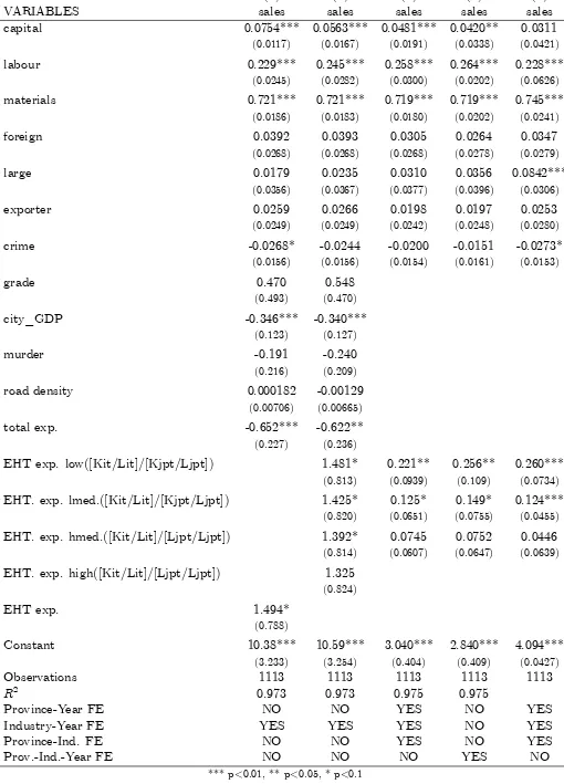
constant and capture the e¤ects of increasing EHT expenditure as a share of total expenditure on …rm sales.

Starting with the control variables we …nd that the production function performs sensibly and the estimated elasticities (calculated at the means of the other right-hand side variables) are within the expected range. The elasticity with respect to physical capital and labor in regression (1) are 0.075 and 0.229 respectively and there are mildly increasing returns across all of the private inputs for the …rms in our sample. Of the …rm and province-level variables only the crime variable and the city_GDP variables are statistically signi…cant at conventional levels, with the latter having a surprising negative e¤ect on …rm productivity. This may indicate that there are congestion e¤ects in large cities which lower productivity.

Turning next to the …scal variables, the estimated coe¢ cient for total expenditure is negative and statistically signi…cant. Using the Barro (1990) model to interpret this result would imply that the level of government ex-penditure is beyond the optimal point in South Africa, such that the negative e¤ects of taxation on growth outweigh any positive e¤ects that expenditures might have. For the main variable of interest, the share of EHT spending, we …nd that this has a positive relationship with …rm sales (with signi…cance at the 10% level), suggesting that changes to the expenditure mix is associated with rising productivity on average.

Regression 2 in Table 5 refers to our baseline estimation of hypothesis (2) and captures alongside the e¤ect of changes to total government spending the possibility that they di¤er across …rms with di¤erent capital-labor ratios. Note that the capital-labor ratio of the …rm is measured relative to the mean in each individual industry, province and time period. In all regressions we continue to control for shocks to industries using a full set of industry-time dummies and use province-industry clustered standard errors to control for intra-class correlation.8

For the e¤ects of EHT expenditure, we …nd evidence of an interesting di¤erence in its e¤ect across …rms. The coe¢ cients for this variable can be interpreted as the e¤ect on …rm-level productivity of an increase in the EHT share compensated by a pro-rata decrease in other types of public spending, leaving total province expenditures constant. The results indicate that such a change to …scal policy would increase productivity for …rms with all but the highest capital-labor ratios with signi…cance at the 10% level, for whom we …nd no e¤ect at least over the short-run. As already noted this could

8_{The number of provinces is too small to cluster at the provincial level only. To further}

imply either that there is no e¤ect from changes to the expenditure mix for these …rms, or that the compensating items have an e¤ect that o¤sets the e¤ect of increased EHT spending for these …rms.

In regression (3) we account for the e¤ect of time-varying province as well as time-invariant province-industry characteristics that have been omitted from regression (2). The former might include province-speci…c components of the business cycle and policy variables not directly related to …scal policy, while the latter allow for province characteristics such as geography, that might a¤ect the productivity of …rms within an industry compared to those in the same industry and a di¤erent province.

The province-time dummies are of course perfectly collinear with the government expenditure variables, such that the total expenditure variable must be omitted. This also necessitates a change in the way that we include these dummies, and we omit the high capital-labor ratio group, such that we now test for di¤erences in the e¤ects of …scal policy relative to the reference category.

The results from regression (3) now indicate that half of South-African …rms are a¤ected by changes to the expenditure mix (with signi…cance at the 5% and 10% level, respectively). As in regression (2) we …nd that the productivity of those …rms with the low and lower medium capital labor ratios are a¤ected by changes to the expenditure mix. A strict interpretation of the results from this regression would be that …rms which use relatively less (low and lower medium) capital to labor in production are a¤ected di¤erently compared to …rms with other capital-labor ratios from increasing the share of spending on EHT within total …scal expenditures over the short-run. If, as implied by the results from regression (2), the productivity of those …rms with the highest capital-labor ratios is una¤ected by these changes to the expenditure mix, then this interpretation might be further strengthened to say that the productivity of low capital-labor ratio …rms is increased. We continue to make this assumption throughout the rest of the paper.

ex-plore whether there are alternative changes to the expenditure mix that would stimulate the productivity of high capital-labor …rms. We consider this question in more detail in Table 7, using the remaining regressions in Section 5 to explore the robustness of the initial …ndings.

As already highlighted an important concern is whether our results cap-ture the e¤ect of unobservable province-industry time-varying factors that a¤ect both the productivity of …rms within a province and the mix of …s-cal expenditures. In the absence of suitable variables to instrument for the expenditure mix within a province, we continue with the practice started in regression (3) of adding further control variables. This allows us to at least judge how important omitted variables are likely to be for the results that we …nd. In regression (3) we included a full set of year and province-industry dummies. In regression (4) we develop this further and control for the possibility that there are shocks that occur at the province-industry-time level that a¤ect productivity and the expenditure variables. The e¤ect of the changes to the expenditure mix are therefore identi…ed in this regression from di¤erences in the e¤ect of policy across …rms within the same province, industry and year.

Despite the demanding nature of this identi…cation strategy we …nd that our results are left unchanged. We continue to …nd evidence that those …rms that have a low or a medium-low ratio of capital to labor relative to other …rms in their industry in that province are a¤ected by shifting the expen-diture mix compared to high K/L …rms. We also …nd that the magnitude of these e¤ects are very similar to those from regression (3), suggesting that omitted province-industry-time e¤ects were not an important explanation for the results in the earlier regressions.

5

Robustness of the Results

5.1

Endogeneity of Private Inputs and the Clustering

of the Standard Errors

In order to exploit the full four years of …rm data, we proceed by esti-mating (5) in two steps. In the …rst step we estimate equation (5) including all four years of available data. In this step, we include …rm …xed e¤ects and province-year e¤ects for 2002 and 2006, to avoid any bias caused by omitting the remaining variables (including the …scal variables) from this regression.9

In the second step we impose the coe¢ cients on the private input variables estimated in step 1 and then re-estimate the model including the …rm and …scal variables that were omitted from the …rst stage. We hope from this exercise to improve the precision with which we estimate the coe¢ cients on the input variables.

In regression (5) of Table 5, we report the results from the two-stage es-timation where the …rst stage is estimated using …rm …xed e¤ects. Again the results are robust to this point.10 _{In the two-stage estimation results}

we continue to …nd that the coe¢ cients on the …scal variables are statisti-cally signi…cant and that the estimated elasticities are largely unchanged. Changing the mix of province-level expenditures towards EHT spending cat-egories whilst holding the total budget constant, is associated with changes in …rm-level output for …rms with a low capital intensity.11

Another concern relates to the clustering of the standard errors. In re-gression (1) Table 6 we therefore use the wild cluster bootstrap estimator proposed by Cameron et al. (2008) to further control for intra-class correla-tion at the province and industry level. In this speci…cacorrela-tion, we are only able to include province-year e¤ects. The coe¢ cient on the share of EHT expen-diture for …rms with a low capital intensity remains signi…cant and robust, although their magnitude decreases.

5.2

Categorization of Firms and Unobserved Firm-Level

Characteristics

Thus far we have used di¤erences in the relative factor intensity of capital and labor of …rms to identify the e¤ects of changes to the public expenditure mix on productivity performance. The decision to express these capital-labor ratios relative to the mean value in each industry, province and year, along with the province-time and province-industry dummies that we include, en-sures that our results cannot be explained by di¤erences in the characteristics

9_{Given that the location of …rms in 2000 and 2001 is unknown, we cannot include}

province-year e¤ects in these regressions. As a robustness check, we also ran regressions with no province-year e¤ects and with province-year e¤ects for all years.

10_{The standard errors of the output elasticities with respect to the private inputs come}

from the …rst stage.

of particular industries, or because province-speci…c di¤erences in relative in-put prices lead to di¤erent factor intensities across provinces. Along similar lines, our results cannot re‡ect the decision by an entrepreneur to open a …rm producing a particular type of product in a particular province because the expenditure mix in that province favors a production technology of that type. Such e¤ects will instead be re‡ected in the mean value of the capital-labor ratio.

The possibility that other …rm characteristics might explain our results, or may also be important, remains however. For example, if larger …rms tend to be on average more capital intensive than smaller …rms, then it might be the relative size of …rm, rather than capital-labor intensity, that is impor-tant. Alternatively, it is now well established in the international economics literature that exporters are larger and more productive than …rms that serve the domestic market only and they may therefore respond to changes in the expenditure mix di¤erently.

In speci…cation (2) in Table 6 we report the results when including in-teractions between the export status of the …rms and the share of EHT expenditure alongside the versions based on the capital-labor ratio. The re-sults show that the export status has no signi…cant e¤ect for the relationship with the change in the spending mix that we examine.12

In regressions (3) and (4) in Table 6 we explore whether the size of the …rm a¤ects the relationship with changes to the mix of public spending, which we measure by the amount of labor, relative to the province-industry mean, and the size of the capital stock, measured relative to the province-industry mean (we retain the labelling of low,lmed and hmed).

We do not …nd that the share of EHT expenditures matters for any of these types of …rms. Firms that are small, or medium sized, when measured by either the amount of labor or capital they possess, are not signi…cantly a¤ected by an increase in EHT spending compensated by a decrease in other types of spending. We conclude from this exercise that the capital-labor ratio successfully captures which …rms are a¤ected by changes to …scal policy that we examine.

As an additional exercise, we test whether our results are driven by the particular way in which we group …rms based on their relative capital-labor intensity. In speci…cation (5), instead of using quartiles, we use quintiles of the distribution of capital-labor across …rms. In speci…cation (5) we continue to …nd that the e¤ects of the share of EHT spending are signi…cant for the bottom groups.13

12_{We do not rule out the possibility that this type of interaction helps to identify an}

e¤ect for a change in spending we have not considered.

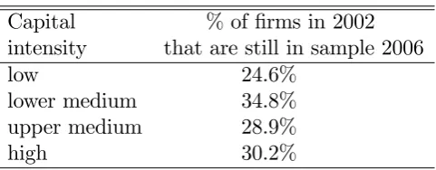
Table 4: Attrition rates

Capital % of …rms in 2002 intensity that are still in sample 2006

low 24.6%

lower medium 34.8% upper medium 28.9%

high 30.2%

Another concern is that we insu¢ ciently control for unobserved …rm-level characteristics. While we control for …rm …xed e¤ects in the …rst step of the two-stage speci…cations, in speci…cation (1) of Table 7, we also add …rm …xed e¤ects. Even though we only have two years of data which is the reason why we normally do not use …rm …xed e¤ects at this stage in the remaining speci…cations, our results remain robust.

Finally, there may be a concern about the classi…cation of …rms as our panel is unbalanced. If capital intensity is correlated with productivity, then …rm exit rates can assumed to be highest in the low capital-intensity group and lowest in the high capital-intensity group. This would imply that the panel is not unbalanced for idiosyncratic reasons which may bias the results. In our sample, we de…ne attrition as …rms that are included in the sample in the 2002 wave but not in the 2006 wave.14 _{Attrition rates do indeed di¤er}

between the groups, and they are highest in the low capital-labor group. However, there does not appear to be a systematic pattern, as they are by far lowest in the medium capital intensity group. The di¤erence in attrition rates between the low-capital intensity group and the omitted capital intensity group (which may have the highest productivity according to this reasoning) is about six percentage points and therefore relatively small. Table 4 provides details.15

capital intensities (not shown).

14_{By construction of the …rm-level data, there is no attrition prior to 2002 as the panel}

dimension for 2000 and 2001 is constructed from the 2002 questionnaire only. In addition, we do not observe attrition after 2006.

15_{When we only include …rms with observations in 2002 and 2006 in speci…cation (1)}

5.3

De…nition of Public Expenditure and Exogeneity

of its Composition

The richness of the public spending data for South Africa throws up an interesting question, namely of whether there are alternative changes to the mix of public spending that a¤ect the productivity of …rms, and whether or not those …rms with low and medium-low capital intensity are a¤ected by these changes. As explained above, given our de…nition of the expenditure mix this will depend on the choice of …scal expenditures that are assumed to increase as well as which ones are assumed to decrease to compensate for this. We use this section of the paper to explore issues relating to our categorization of public spending.

We begin with some discussion of the denominator of the EHT variable, which includes the remaining province-level public spending. Even though we take averages of public spending over two years, it is conceivable that the denominator of the spending share variable co-moves with the business cycle because it includes transfers or other expenditures that exhibit pro-cyclical behavior. While correlations between regional growth rates and the public spending shares we construct indicates that this is unlikely (the correlation coe¢ cient between the annual share of EHT spending and provincial growth is below 0.25 and statistically not di¤erent from zero), speci…cation (2) of Table 7 considers this more formally.

In regression (2) of Table 7 we express EHT expenditure as a share of total expenditure on education, health and transport sectors (i.e., the de-nominator also includes for instance administrative spending within these categories, but no spending outside these categories). The results from this regression suggest that reallocating resources within total education, health and transport spending also a¤ects the productivity of …rms according to their capital-labor ratio. Again we …nd no productivity response for …rms with a capital-labor ratio above this.

In speci…cation (3), we develop this idea further and exclude both spend-ing on emergency care and on public works from the denominator. A pos-sibility exists that these expenditure categories have a di¤erent sensitivity to cyclical ‡uctuations compared to the remaining expenditure items. For political reasons, emergency care spending may be safeguarded from cuts and remain fairly stable over the cycle, while in contrast, public works are subject to long planning and execution cycles. Speci…cation (3) now suggests that only the productivity of those …rms with the lowest capital-labor ratios would be a¤ected by increasing this spending ratio.

of education, health and public infrastructure and transportation that may be expected to be productive over the short run. When we include all subcate-gories of health, education as well as public infrastructure and transportation, where this now includes expenditures on administration, in speci…cation (4) of Table 7, the coe¢ cient of the share of EHT expenditure is again statisti-cally signi…cant for …rms with low and medium-low capital-labor ratios.

In speci…cation (5), we take the alternative approach and are more selec-tive in the subcategories of education, health as well as public infrastructure and transportation spending we include. In this regression we include in the numerator expenditure on early childhood development, district health services and spending on public transportation only. The coe¢ cients for medium-low and low K/L are much reduced in size, but remain positive and signi…cant in these regressions. It is also noticeable that the estimated coe¢ -cients are much smaller than those found up until this point, suggesting that while signi…cant the relative productivity changes they cause across …rms are comparatively small compared to other changes to the expenditure mix.

As a …nal exercise we include education, health and transport as separate categories and express them as a ratio to total EHT expenditure. These are reported in regressions (1), (2) and (3) in Table 8. Interestingly we now …nd a signi…cant productivity e¤ect only for health and transport spending for low and medium-low capital labor ratio …rms. As already noted, this does not necessarily imply there are no productivity e¤ects from changes to education expenditure as they may be o¤set by the other compensating changes that occur in order to leave total expenditure constant. It does at least indicate that low K/L …rms are not always a¤ected by changes to the expenditure mix in a way that is di¤erent from …rms with higher K/L ratios.

6

Conclusions

that low K/L …rms bene…t from changes to the expenditure mix as their productivity rises in contrast to more capital intensive …rms.

We conclude from the evidence we present that governments are able to a¤ect …rm productivity by reallocating public spending. Given that pro-ductivity at the …rm level is likely to be fundamental for long-run aggregate economic growth, changes to the expenditure mix may be less expensive than raising total public spending and therefore raising additional revenues. This is of current relevance given the large budget de…cits due to the recent eco-nomic crisis in many countries. Second, if governments attempt to raise …rm productivity via the reallocation of public resources, our results indicate that it is important that they take into account the characteristics of …rms. While this issue needs to be further explored in future research, our results indicate that these e¤ects depend on the technology of …rms that in turn drive their capital intensities.

We leave several possible extensions for future work. The robustness of the results could be further tested through the use of additional estimators and empirical methods. Our identi…cation strategy addresses endogeneity in a manner that is similar to many other papers using macro and micro level data, but concerns over the direction of causation therefore still remain. There are also other aspects of the dataset that could be exploited further. For instance, it would be possible to compare the e¤ects of aggregate EHT spending when o¤set by di¤erent elements of the government budget, and it would be possible to explore the role of additional …rm characteristics for the e¤ects of public spending.

Table 5: Results

(1) (2) (3) (4) (5) VARIABLES sales sales sales sales sales capital 0.0754*** 0.0563*** 0.0481*** 0.0420** 0.0311

(0.0117) (0.0167) (0.0191) (0.0338) (0.0421)

labour 0.229*** 0.245*** 0.258*** 0.264*** 0.228***

(0.0245) (0.0282) (0.0300) (0.0202) (0.0626)

materials 0.721*** 0.721*** 0.719*** 0.719*** 0.745***

(0.0186) (0.0183) (0.0180) (0.0202) (0.0241)

foreign 0.0392 0.0393 0.0305 0.0264 0.0347

(0.0268) (0.0268) (0.0268) (0.0278) (0.0279)

large 0.0179 0.0235 0.0310 0.0356 0.0842***

(0.0356) (0.0367) (0.0377) (0.0396) (0.0306)

exporter 0.0259 0.0266 0.0198 0.0197 0.0253

(0.0249) (0.0249) (0.0242) (0.0248) (0.0280)

crime -0.0268* -0.0244 -0.0200 -0.0151 -0.0273*

(0.0156) (0.0156) (0.0154) (0.0161) (0.0153)

grade 0.470 0.548

(0.493) (0.470)

city_GDP -0.346*** -0.340***

(0.123) (0.127)

murder -0.191 -0.240

(0.216) (0.209)

road density 0.000182 -0.00129

(0.00706) (0.00665)

total exp. -0.652*** -0.622**

(0.227) (0.236)

EHT exp. low([Kit/Lit]/[Kjpt/Ljpt]) 1.481* 0.221** 0.256** 0.260***

(0.813) (0.0939) (0.109) (0.0734)

EHT. exp. lmed.([Kit/Lit]/[Kjpt/Ljpt]) 1.425* 0.125* 0.149* 0.124***

(0.820) (0.0651) (0.0755) (0.0455)

EHT. exp. hmed.([Kit/Lit]/[Ljpt/Ljpt]) 1.392* 0.0745 0.0752 0.0446

(0.814) (0.0607) (0.0647) (0.0639)

EHT. exp. high([Kit/Lit]/[Ljpt/Ljpt]) 1.325

(0.824)

EHT exp. 1.494*

(0.788)

Constant 10.38*** 10.59*** 3.040*** 2.840*** 4.094***

(3.233) (3.254) (0.404) (0.409) (0.0427)

Observations 1113 1113 1113 1113 1113

R2 _{0.973 0.973 0.975 0.975}

Province-Year FE NO NO YES NO YES

Industry-Year FE YES YES YES NO YES

Province-Ind. FE NO NO YES NO YES

Prov.-Ind.-Year FE NO NO NO YES NO

*** p<0.01, ** p<0.05, * p<0.1

Table 6: Robustness I

(1) (2) (3) (4) (5) VARIABLES sales sales sales sales sales

capital 0.0585 0.0482*** 0.0755*** 0.0576*** 0.0474***

(0.0180) (0.0120) (0.0194) (0.0180)

labour 0.253 0.258*** 0.244*** 0.232*** 0.259***

(0.0190) (0.0282) (0.0251) (0.0191)

materials 0.714 0.719*** 0.720*** 0.718*** 0.719***

(0.0301) (0.0198) (0.0195) (0.0303)

foreign 0.0509*** 0.0308 0.0280 0.0295 0.0302

(0.0269) (0.0276) (0.0270) (0.0273)

large -0.00309 0.0311 0.0277 0.0238 0.0313

(0.0376) (0.0330) (0.0369) (0.0376)

exporter 0.0392 0.0192 0.0202 0.0197

(0.0241) (0.0248) (0.0243)

crime -0.0270*** -0.0199 -0.0207 -0.0194 -0.0201

(0.0154) (0.0152) (0.0149) (0.0155)

EHT exp. low 0.149*** 0.220** -0.0845 0.198 0.227**

(0.0939) (0.126) (0.138) (0.0970)

EHT exp. lmed. 0.0939*** 0.124* 0.00714 0.141 0.130*

(0.0652) (0.0791) (0.105) (0.0659)

EHT exp. hmed. 0.0722 0.0742 0.0196 0.0531 0.0789

(0.0606) (0.0576) (0.0698) (0.0544)

EHT exp. high 0.0141

(0.0758)

EHT exp. [exporter] -0.0253

(0.0325)

Constant 2.859*** 3.034*** 2.016*** 3.174*** 3.041***

(0.773) (0.404) (0.446) (0.423) (0.403)

Observations 1,113 1,113 1,113 1,113 1,113

R2 0.970 0.975 0.975 0.975 0.975 Province-Year FE YES YES YES YES YES Industry-Year FE NO YES YES YES YES Province-Ind. FE NO YES YES YES YES Prov.-Ind.-Year FE NO NO NO NO

*** p<0.01, ** p<0.05, * p<0.1

ind.-prov. clustered standard errors in parentheses OLS estimates based on 2002 and 2006.

Table 7: Robustness II

(1) (2) (3) (4) (5) VARIABLES sales sales sales sales sales

capital -0.00379 0.0510*** 0.0509*** 0.0494*** 0.0484***

(0.0306) (0.0296) (0.0304) (0.0192) (0.0185)

labour 0.448*** 0.255*** 0.254*** 0.258*** 0.258***

(0.0876) (0.0181) (0.0183) (0.0171) (0.0191)

materials 0.697*** 0.719*** 0.720*** 0.719*** 0.719***

(0.0303) (0.0190) (0.0192) (0.0301) (0.0302)

foreign -0.0355 0.0306 0.0322 0.0300 0.0309

(0.102) (0.0268) (0.0268) (0.0268) (0.0269)

large -0.0354 0.0306 0.0328 0.0301 0.0290

(0.151) (0.0379) (0.0387) (0.0375) (0.0377)

exporter -0.0515 0.0197 0.0192 0.0199 0.0201

(0.0841) (0.0244) (0.0245) (0.0242) (0.0242)

crime 0.0223 -0.0205 -0.0197 -0.0195 -0.0203

(0.0412) (0.0154) (0.0156) (0.0154) (0.0154)

EHT exp. low([Kit/Lit]/[Kjpt/Ljpt]) 0.450*** 0.308* 0.369* 0.587*** 0.0541**

(0.105) (0.155) (0.202) (0.219) (0.0244)

EHT exp. lmed.([Kit/Lit]/[Kjpt/Ljpt]) 0.303*** 0.175 0.223 0.326** 0.0304*

(0.0788) (0.107) (0.141) (0.159) (0.0166)

EHT exp. hmed.([Kit/Lit]/[Ljpt/Ljpt]) -0.0150 0.109 0.123 0.179 0.0211

(0.128) (0.0991) (0.126) (0.148) (0.0160)

Constant 4.440*** 3.021*** 3.010*** 3.048*** 3.062***

(0.950) (0.403) (0.383) (0.405) (0.402)

Observations 1,113 1,113 1,095 1,113 1,113

R2 _{0.966 0.975 0.975 0.975 0.975}

Number of eec_panelid 981

Province-Year FE YES YES YES YES YES Industry-Year FE YES YES YES YES YES Province-Ind. FE YES YES YES YES YES

Firm FE YES NO NO NO NO

*** p<0.01, ** p<0.05, * p<0.1

ind.-prov. clustered standard errors in parentheses OLS estimates based on 2002 and 2006

(1) Firm …xed e¤ects added

(2) EHT exp. as a ratio of all exp. in these categories

(3) same as (2) except that emergency and public works is excluded from denominator (4) broad de…nition of EHT expenditure used

Table 8: Robustness III

(1) (2) (3) VARIABLES sales sales sales

capital 0.0581*** 0.0519*** 0.0487***

(0.0183) (0.0183) (0.0304)

labour 0.249*** 0.255*** 0.258***

(0.0287) (0.0191) (0.0191)

materials 0.719*** 0.719*** 0.719***

(0.0192) (0.0300) (0.0182)

foreign 0.0309 0.0309 0.0310

(0.0270) (0.0270) (0.0270)

large 0.0253 0.0279 0.0280

(0.0379) (0.0376) (0.0375)

exporter 0.0205 0.0202 0.0206

(0.0244) (0.0243) (0.0243)

crime -0.0205 -0.0204 -0.0204

(0.0153) (0.0154) (0.0154)

EHT exp. low([Kit/Lit]/[Kjpt/Ljpt]) 0.182 0.1000** 0.0530**

(0.113) (0.0482) (0.0237)

EHT exp. lmed.([Kit/Lit]/[Kjpt/Ljpt]) 0.0904 0.0542* 0.0284*

(0.0747) (0.0319) (0.0159)

EHT exp. hmed.([Kit/Lit]/[Ljpt/Ljpt]) 0.100 0.0406 0.0204

(0.0794) (0.0323) (0.0157)

Constant 3.030*** 3.062*** 3.076***

(0.399) (0.404) (0.400)

Observations 1,113 1,113 1,113

R2 _{0.975 0.975 0.975}

Province-Year FE YES YES YES Industry-Year FE YES YES YES Province-Ind. FE YES YES YES

*** p<0.01, ** p<0.05, * p<0.1

ind.-prov. clustered standard errors in parentheses OLS estimation based on 2002 and 2006

A

Appendix

A.1

The System of Fiscal Decentralization in South

Africa

Since the end of the Apartheid era, South Africa has undergone wide-ranging …scal reforms, and a system of transparent, constitutionally compliant inter-governmental …scal relations has been created. Government now comprises three spheres: national, provincial and local. The …scal system departs from conventional prescripts of …scal federalism however because there is a mis-match between expenditure and revenue powers at each of these di¤erent levels of government (Ajam and Aron, 2007).

Public expenditure policy is decentralized in a range of important areas. Provincial governments are largely responsible for spending on provincial roads, education (except higher education), health services, public trans-portation, social welfare services, housing and agriculture. For these func-tions, the level of public spending by the national government is very low, and the national government is mainly responsible for setting minimum norms and standards and for monitoring the overall implementation by provincial governments. It also collects data on provincial public spending (Momoniat, 2002). The expenditure that the national government undertakes can be expected to leave …rm productivity una¤ected over the medium run, or it …-nances public goods such as national roads or higher education and research. In these cases, signi…cant country-wide spillovers imply that there is no or little variation between the provinces. By contrast, provincial governments provide goods and services that are unlikely to entail signi…cant spillovers across provinces.

such as health, infrastructure, housing and social development, and they re-ceive non-earmarked grants (which are referred to as ‘equitable share grants’) (Ajam and Aron, 2007). The level of the latter that a given province receives depends on range of social and economic indicators.

A.2

Industry-Level Descriptive Statistics

Table 9: Distribution of …rms by industry across provinces

industry no. of obs % of obs. % of obs. % of obs.

(2002 - 2006) in KN in GT in WC

Mining & quarrying 3 0.0% 33.3% 66.7% Sale, Maintenance & repair of vehicles 2 0.0% 50.0% 50.0% Manufacture of food & bevarages 154 5.2% 68.2% 18.2% Manufacture of tobacco products 1 0.0% 100.0% 0.0% Manufacture of textiles 21 19.0% 38.1% 33.3% Manufacture of wearing apparel 115 14.8% 57.4% 19.1% Manufacture of luggage & footwear 20 15.0% 70.0% 5.0% Manufacture of wood 49 16.3% 61.2% 20.4% Manufacture of paper 26 19.2% 65.4% 11.5% Publishing, printing & reproduction 47 14.9% 46.8% 38.3% Manufacture of coke & re…ned petroleum 3 0.0% 100.0% 0.0% Manufacture of chemicals 122 8.2% 69.7% 14.8% Manufacture of rubber & plastics 47 8.5% 68.1% 19.1% Manufacture of non-metallic products 25 12.0% 68.0% 20.0% Manufacture of basic metals 20 0.0% 100.0% 0.0% Manufacture of metal products 149 15.4% 69.8% 11.4% Manufacture of machinery 64 4.7% 84.4% 10.9% Manufacture of o¢ ce machinery 2 0.0% 100.0% 0.0% Manufacture of electrical machinery 65 6.2% 84.6% 4.6% Manufacture of motor vehicles 24 12.5% 62.5% 4.2% Manufacture of furniture 150 6.7% 65.3% 22.0%

Recycling 1 0.0% 0.0% 100.0%

Wholesale & retail trade 2 0.0% 100.0% 0.0% Hotels & restuarants 1 0.0% 100.0% 0.0%

all, 2002 - 2006 1113 10.1% 67.7% 16.7%

A.3

Categorization of Public Expenditure

In the empirical speci…cations, we assume that expenditure within education, health, as well as public infrastructure and transportation (EHT) is increased and that this increase is o¤set using expenditure outside these areas and other expenditure on speci…c items within these areas. The underlying assumption is that EHT expenditure a¤ects productivity to a larger extent than the o¤setting expenditure over a period of 1 to 2 years.

Within spending on public infrastructure and transportation referred to as ‘transport expenditure’, we assume that spending on public transport, tra¢ c management and road infrastructure which includes spending on road maintenance can be expected to deliver fairly quickly tangible bene…ts for …rms. For instance, improved tra¢ c lights may cut travel time, …lling pot-holes lowers the cost for repairs, and new bus lines help the work force to reach their workplace more quickly. Spending on public health may also rapidly improves labor productivity, if for instance it results in increased availability of drugs against common diseases, or if public awareness to pre-vent accidents or certain types of diseases increases. We therefore consider spending on district and provincial health services as productive. Here, we expect that public spending may ensure that the work force remains …t for work.

Even spending on education may have almost immediate e¤ects on pro-ductivity: for instance, as a result of education spending on early childhood development, labor productivity of the parents may improve fairly quickly. In addition, improved education of students shortly prior to graduation or spending on short courses for adults may a¤ect labor productivity over the medium run because this type of education is rather short and provides parts of the workforce with skills which are directly relevant for their jobs. We therefore expect that spending on further education and training as well as adult basic education and training as well as spending on public and private schools in general potentially a¤ects private productivity over the medium run.

which are likely to treat many patients who are not part of the work force, at least temporarily. In addition, we exclude emergency medical services which includes emergency and planned patient transport; here the link to …rm-level productivity is also less clear. With respect to education spending, apart from administration, we exclude spending on auxiliary and associated services and on public special school education where the links with private sector productivity are also less direct.

Finally, within the public infrastructure and transportation category, there are a number of areas which are probably less or not relevant at all for …rm productivity. This includes public works which a¤ects productivity at best over longer horizons or not at all (e.g., spending on public works in agriculture which we are unable to separate from spending on public works in say education) and spending on programmes within communities which can expected to have social rather than productive bene…ts.

Table 10 provides an overview of how we categorize public spending. Obviously, we recognize that one could also make alternative choices about which subcategories are considered as productive within the health, educa-tion and public infrastructure and transportaeduca-tion categories. We therefore consider the robustness of the our results to these choices in Section 5.

References

[1] C. Adam and D. Bevan, “Fiscal de…cits and growth in developing coun-tries,”Journal of Public Economics, vol. 89, no. 4, pp. 571–597, 2005.

[2] P. Agénor, “Fiscal policy and endogenous growth with public infrastruc-ture,”Oxford Economic Papers, vol. 60, no. 1, pp. 57–87, 2008a.

[3] — — , “Health and infrastructure in a model of endogenous growth,”

Journal of Macroeconomics, vol. 30, no. 4, pp. 1407–1422, 2008b.

[4] T. Ajam and J. Aron, “Fiscal renaissance in a democratic South Africa,”

Journal of African Economies, vol. 16, no. 5, pp. 745–781, 2007.

[5] J. Arnold, A. Mattoo, and G. Narciso, “Services inputs and …rm produc-tivity in Sub-Saharan Africa: Evidence from …rm-level data,”Journal

Table 10: Fiscal variables provided by the South African Treasury

Variable Description (all in logs)

total expenditure total provincial expenditure / GDP

health expenditure, education EHT expenditure expenditure,transport &

capital expenditure

public ordinary school education, independent school subsidies, Education expenditure further education and training, adult basic training,

early childhood development

Health expenditure district health services, provincial hospital services Transport & capital exp. road infrastructure, public transport, tra¢ c management

mainly agriculture, social development, housing, sport, recreation, arts and culture, administration,

education (only public special school education, auxiliary and associated services)

Other expenditure health (emergency medical services, central hospital services, (o¤setting categories) health sciences and training, health care support services,

health facilities management)

[6] B. H. Baltagi and N. Pinnoi, “Public capital stock and state productivity growth: further evidence from an error components model,”Empirical

Economics, vol. 20, no. 2, pp. 351–359, 1995.

[7] R. Barro, “Government spending in a simple model of economic growth,”

Journal of Political Economy, vol. 98, no. 5, pp. 103–25, 1990.

[8] F. Bastos and J. Nasir, “Productivity and the Investment Climate: What Matters Most?” World Bank Policy Research Paper, no. 3335, 2004.

[9] G. Bekes and B. Murakozy, “Firm Behaviour and Public Infrastructure: The Case of Hungary,”KTI/IE Discussion Papers, no. 4, 2005.

[10] A. Cameron, J. Gelbach, and D. Miller, “Bootstrap-based improvements for inference with clustered errors,”The Review of Economics and

Sta-tistics, vol. 90, no. 3, pp. 414–427, 2008.

[11] S. Datta, “The impact of improved highways on indian …rms,”Journal

of Development Economics, vol. 99, no. 1, pp. 46–57, 2012.

[12] P. David and T. Van de Klundert, “Biased e¢ ciency growth and capital-labor substitution in the U.S., 1899-1960,”The American Economic

Review, pp. 357–394, 1965.

[13] S. Devarajan, V. Swaroop, and H.-f. Zou, “The composition of public expenditure and economic growth,”Journal of Monetary Economics, vol. 37, no. 2, pp. 313–344, 1996.

[14] D. Dollar, M. Hallward-Driemeier, and T. Mengistae, “Investment Cli-mate and Firm Performance in Developing Economies,”Economic

De-velopment and Cultural Change, vol. 54, no. 1, pp. 1–31, 2005.

[15] P. Evans and G. Karras, “Are government activities productive? evi-dence from a panel of us states,”The Review of economics and statistics, pp. 1–11, 1994.

[16] T. Gabe, “Local …scal policy and establishment growth,”Journal of

Regional Analysis and Policy, vol. 33, no. 1, pp. 57–80, 2003.

[17] T. Garcia-Milà and T. J. McGuire, “The contribution of publicly pro-vided inputs to states’ economies,”Regional Science and Urban

[18] N. Gemmell, F. Misch, and B. Moreno-Dodson, “Public spending and long-run growth in practice: Concepts, tools, and evidence,”Is Fiscal

Policy the Answer?: A Developing Country Perspective, p. 69, 2012.

[19] H. Hong and S. Ahmed, “Government spending on public goods: Ev-idence on growth and poverty,”Economic & Political Weekly, vol. 44, no. 31, pp. 103–108, 2009.

[20] R. Kneller, M. Bleaney, and N. Gemmell, “Fiscal policy and growth: evidence from oecd countries,”Journal of Public Economics, vol. 74, no. 2, pp. 171–190, 1999.

[21] J. Levinsohn and A. Petrin, “Estimating production functions using inputs to control for unobservables,”Review of economic studies, vol. 70, no. 2, pp. 317–341, 2003.

[22] J. E. Ligthart and R. M. M. Suárez, “The productivity of public capital: A meta-analysis,” in Infrastructure Productivity Evaluation. Springer, 2011, pp. 5–32.

[23] R. López and S. Miller, “The Structure of Public Expenditure: A Robust Predictor of Economic Development?”Unpublished manuscript, 2007.

[24] K. Mera, “Ii. regional production functions and social overhead capital: An analysis of the japanese case,”Regional and Urban Economics, vol. 3, no. 2, pp. 157–185, 1973.

[25] I. Momoniat, “Fiscal Decentralisation in South Africa: a Practitioner’s Perspective,” in Managing Fiscal Decentralization, E. Ahmad and V. Tanzi, Eds. Routledge, 2002, pp. 350–374.

[26] R. Reinikka and J. Svensson, “Coping with poor public capital,”Journal

of Development Economics, vol. 69, no. 1, pp. 51–70, 2002.

[27] D. Rodrik, “The debate over globalization: how to move forward by looking backward,”Launching new global trade talks: an action agenda, p. 25, 1998.

[29] C. Schwellnus and J. Arnold, “Do Corporate Taxes Reduce Productivity and Investment at the Firm Level? Cross-country Evidence from the Amadeus Dataset,”OECD Economics Department Working Papers, no. 641, 2008.

[30] C. Shirley and C. Winston, “Firm inventory behavior and the returns from highway infrastructure investments,”Journal of Urban Economics, vol. 55, no. 2, pp. 398–415, 2004.

[31] S. Straub, “Infrastructure and Growth in Developing Countries: Re-cent Advances and Research Challenges,”World Bank Policy Research