Habitat preferences and distribution of harbour porpoise (Phocoena phocoena) west of Scotland

INTRODUCTION

The harbour porpoise Phocoena phocoena is a small odontocete, which is widely distributed through -out both the Atlantic and Pacific temperate and sub-arctic regions of the Northern Hemisphere (Evans 1980). It is the most common cetacean species on the west coast of Scotland, where year-round sightings have been reported (Reid et al. 2003). Harbour por-poises are mainly found in inshore continental shelf waters (CODA 2009, Marubini et al. 2009, Embling et al. 2010), and the west coast of Scotland has one of the highest densities of porpoises in Europe (SCANS-II 2008).

The majority of cetacean distribution studies have used boat-based or aerial visual surveys as the

pri-mary data collection method (SCANS-II 2008, Gilles et al. 2011, Scheidat et al. 2012). In the case of species that are difficult to detect visually, such as the har-bour porpoise, visual surveys are heavily impacted by survey vessel speeds (Embling et al. 2010) and sea state (i.e. sightings decrease as Beaufort sea states in crease >1: Palka 1996, Teilmann 2003). Another increasingly popular method of studying porpoises is Passive Acoustic Monitoring (PAM) (Gillespie et al. 2005, Embling 2007, Sveegaard et al. 2011); towed PAM systems have previously been used to comple-ment visual survey methods (Gillespie et al. 2005, CODA 2009, SCANS-II 2008).

Predictive or explanatory modelling is a widely used method of identifying the key factors driving habitat preferences for a species. This type of

model-© Inter-Research 2013 · www.int-res.com *Email: cgb@smru.co.uk

Habitat preferences and distribution of the harbour

porpoise

Phocoena phocoena

west of Scotland

C. G. Booth

*, C. Embling

_{, J. Gordon}

_{, S. V. Calderan}

_{, P. S. Hammond}

1_{Sea Mammal Research Unit, Scottish Oceans Institute, University of St Andrews, St Andrews, Fife KY16 8LB, UK} 2_{Centre for Ecology and Conservation, University of Exeter, Cornwall Campus, Penryn TR10 9EZ, UK}

3_{Marine Ecological Research Ltd., Newport-on-Tay, Fife DD6 8JH, UK}

4_{Hebridean Whale and Dolphin Trust, 28 Main Street, Tobermory, Isle of Mull PA75 6NU, UK}

ABSTRACT: The west coast of Scotland is comprised of complex coastlines and topography, and a range of physical processes influence its coastal marine environment. The region is host to one of the highest densities of harbour porpoise Phocoena phocoenain Europe. The aim of this study was to identify habitat preferences driving the distribution of harbour porpoise, to gain a better under-standing of the spatial distribution of the species in the region, as well as to assess the consistency of such patterns across time and space. Visual and acoustic line-transect surveys were conducted between 2003 and 2010. Generalised Additive Models (GAMs) with Generalised Estimating Equations (GEEs) were used to robustly determine relationships between the relative density of harbour porpoises and temporally and spatially variable oceanographic covariates. Predictive models showed that depth, slope, spring tidal range and distance to land were consistently impor-tant in explaining porpoise distribution. Consistent preferences for water depths between 50 and 150 m and highly sloped regions were observed across the temporal models. Predicted distribu-tions revealed a consistent inshore presence for the species throughout the west coast of Scotland and confirmed that predictable oceanographic features could help inform the establishment of Special Areas of Conservation (SACs) for the species.

KEY WORDS: Harbour porpoise · Habitat preference · Distribution · Interannual variability

ing has been used successfully for harbour porpoises (Tynan et al. 2005, Bailey & Thompson 2009, Embling et al. 2010). It is likely that the distribution of por-poises is strongly influenced by the abundance and distribution of its prey (as high consumption rates must be achieved daily to meet their energetic needs; Read & Westgate 1997, Lockyer 2007) and its preda-tors (Heithaus & Dill 2006). Direct links have been observed between porpoise distribution and that of their prey (Sveegaard et al. 2012a,b). However, such direct data are difficult to obtain, especially at an appropriate temporal or spatial scale. In their ab -sence, many studies have used indirect factors that are easier to measure to serve as proxies for the direct factors, e.g. seabed depth and slope (Bailey & Thompson 2009, Marubini et al. 2009, Isojunno et al. 2012), sediment (Edrén et al. 2010, Embling et al. 2010) and tidal cycles (Johnston et al. 2005, Pierpoint 2008, Embling et al. 2010).

The harbour porpoise is listed on Annex II of the Habitats Directive (Council Directive 92/43/EC), which requires member states to set up Special Areas for Conservation (SACs) for the species. However, no SACs have been designated for harbour porpoise in the UK, in part due the highly mobile nature of the species, although sites have been designated in other parts of Europe.

In this paper, we present a comprehensive and robust investigation of the key environmental drivers influencing the distribution of harbour porpoises west of Scotland, using models populated with data from boat-based surveys conducted between 2003 and 2010. Visual and acoustic survey data were mod-elled with respect to a range of survey, environmen-tal and oceanographic-proxy data to determine if there were consistent patterns. Using the outputs of these models, we predicted relative spatial distribu-tion patterns for porpoises across the west coast of Scotland to highlight potential areas of importance for the species that could help inform the SAC selec-tion process.

MATERIALS AND METHODS

Systematic surveys (both line-transect visual and acoustic towed hydrophone) were carried out from the Hebridean Whale and Dolphin Trust’s 18 m motor-sailor vessel ‘Silurian’ between 2003 and 2010 (visual only in 2003). Every month between April and September, at least one 10 d daylight survey was conducted covering a portion of the study area, fol-lowing a systematic zig-zag pattern to ensure that

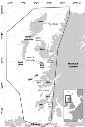
the study area was surveyed as evenly as possible within the constraints of the weather and local ports. The west coast of Scotland is a hydrographically diverse region. It is topographically complex with numerous fjordic sea lochs and deep (> 200 m) steep-sided submarine canyons coupled with several islands, inlets and channels that provide a wide range of environments and sea conditions (Ellett & Edwards 1983; Fig. 1). In coastal waters depth is variable, although further offshore depth generally increases as a function of distance from land, and seabed slopes are shallower. Tidal range varies throughout the study region. Some areas have large tidal ranges, generating high current speeds (Gilli-brand et al. 2003, Inall et al. 2009); the largest tidal ranges are around the Isle of Skye and the Minch. Most areas have tidal ranges of > 2 m. The notable exception is the Sound of Jura in the south of the region, where the tidal range drops as a result of 2 water masses (Irish Sea and Atlantic flow) being 180° out of phase and converging in the region (see Gilli-brand et al. 2003). The varying tidal ranges across the region make it desirable to design habitat models with dynamic and fixed covariates.

Visual surveys

Visual surveys were carried out by teams of 2 observers positioned on the front deck (eye height: 3 m). Each observer surveyed one side each from 0° (ahead of the vessel) to 90° (abeam of the vessel) with the naked eye and 7 × 50 binoculars (Marine Opticron and Plastimo). Observers were rotated every hour to avoid fatigue. When a porpoise was sighted, we recorded the time, group size, estimated range to the animal(s), the bearing to the animal(s) relative to the boat (determined from angle boards on deck) as well as the behavior of the animal. Envi-ronmental, survey and effort data were entered into the software Logger 2000 (IFAW/ Doug Gillespie), which continuously logged vessel and navigational data.

Acoustic surveys

Rainbow Click (a pre-cursor to the PAMGUARD porpoise click detector) from 2006 to 2010. These systems used different hydrophone arrays and differ-ent software for signal processing and acoustic detection. Both hydrophone arrays were comprised of 2 high-frequency elements (HS150 elements; Sonar Research & Development) with the highest sensitivity at 150 kHz, and a near flat frequency response between 2−140 kHz. In 2004 and 2005, the hydrophone elements were separated by 3 m, where -as in 2006 through 2010 they were separated by 0.25 m. Both hydrophone arrays were towed 100 m behind the boat attached by Kevlar-strengthened towing cable.

Data collected using Porpoise Detector (Version 4.00.0001; Gillespie & Chappell 2002) in 2004 and 2005 were analysed by Embling (2007). Embling’s methods used the Porpoise Detector software to automatically classify clicks as porpoises. Porpoise click events were classified as a ‘porpoise click train’ if the clicks had a minimum amplitude of >105 dB re 1 µPa in the porpoise frequency band (115−145 kHz) and there was a > 30 dB difference above the mean amplitude in both control (50 and 71 kHz) bands. Detection data collected using Rainbow Click (Version 4.04.0001; IFAW/Doug Gillespie) were auto-matically identified and verified using the same methodology employed in the SCANS-II acoustic analysis (Swift et al. 2008).

For all porpoise clicks, a bearing to the source was calculated (with a left/right ambi-guity) by measuring the difference in time of arrival between one hydrophone and the other. The number of porpoises per group was estimated based on the number of click events/trains detected simultaneously. All porpoise detections during the study were analysed by a manual operator independ-ently of the visual data to remove false posi-tives. It should be noted that some technical issues were encountered during the 2009 sur-vey season. As 2 PAM systems were used in this study, the detection system that was used was included as a candidate covariate in the model selection process.

Sources of covariate data

A range of survey covariates was included in models to account for patterns in the data driven by the methods used (Table 1). For visual sur-veys, only efforts conducted in Beaufort sea state ≤3 were used, whereas for acoustic surveys efforts in all sea states (0−6) were included. Survey efforts con-ducted in poor weather conditions (e.g. fog, heavy rain, ex treme glare) were excluded from further analyses. The total number of detections in each 2 km survey segment (the response variable) was cal-culated. Vessel speed and engine status (i.e. on or off), as well as the PAM system used were also included as candidate covariates.

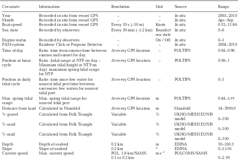
neap) and position in the daily tidal cycle were all included in the models as continuous indices between 0 and 1 in order to incorporate diurnal and tidal temporal variations in the data. Tidal and sun-rise/sunset data were sourced from POLTIPS (Ver-sion 3.0, Proudman Oceanographic Laboratory); the nearest tidal port and distance to land for each data point was determined using Manifold (Version 8.00). Current speed data were obtained from the POL-COMS CS20 model. Sediment data were obtained primarily from United Kingdom Hydrographic Office (UKHO); for regions not covered by those data, the Marine European Seabed Habitats (MESH) EUNIS model was used. Bathymetry data (average seabed depth and slope) were sourced from EDINA (0.2 × 0.2 km grid). Average slope (the change in depth over the resolution of the grid) was determined in Mani-fold. Sea surface temperature and satellite-derived chlorophyll levels were not included in the analyses as they were not available a suitable resolution.

Data analysis

Pre-statistical analysis

Data collected when the survey team was ‘off-effort’ were excluded from the analysis and all remaining visual and acoustic survey effort track-lines were divided into 2 km segments for analysis. ‘Left-over’ effort of less than 2 km was excluded. This exclusion is unlikely to have caused any significant bias in the data as this effort typically corresponded with the end of the survey day, when the survey ves-sel was very close to shore where there were few available covariate data (and thus would have been excluded at the model selection stage). This segment length was determined by the coarsest resolution of the available oceanographic covariates in the mod-els. Prior to segmenting, values for predictor vari-ables were determined for each GPS data point of trackline (at least every 10 s of effort). Where no Covariate Information Resolution Unit Source Range Year Recorded in situfrom vessel GPS – – In situ 2003−2010 Month Recorded in situfrom vessel GPS – – In situ Apr−Sep Boat speed Recorded in situfrom vessel GPS Every 10 s (∼30 m) Knots In situ 0.72−11.86 Sea state Recorded by observers Every 30 min (∼5.2 km) Beaufort In situ 0−6

sea state

Engine status Recorded by observers – On / Off In situ 0−1 PAM system Rainbow Click or Porpoise Detector – – In situ 2004−2010 Time of day Ratio: time from sunrise:time between At every GPS location – POLTIPS 0.04−0.96 sunrise and sunset for day

Position in lunar Ratio: (tidal range at NTP on day − At every GPS location – POLTIPS 0.08−1 cycle Minimum tidal height at NTP on

day): maximum spring tidal range

for NTP Position in daily Ratio: time since low water for At every GPS location – POLTIPS 0−1 tidal cycle nearest tidal port:time between

successive low waters for nearest

tidal port

Max. spring tidal Max. spring tidal range for At every GPS location m POLTIPS 0.44−5.77 range nearest tidal port

Distance from land Calculated in Manifold At every GPS location m Manifold 14−39 950 % gravel Calculated from Folk Triangle Variable % UKHO/MESH EUNIS

model 0−100 % sand Calculated from Folk Triangle Variable % UKHO/MESH EUNIS

model 0−100 % mud Calculated from Folk Triangle Variable % UKHO/MESH EUNIS

model 0−100 Depth Depth of seabed 0.2 km m EDINA 10−250.3 Slope Slope of seabed 0.2 km ° EDINA 0−15.05 Current speed Max. current speed POL: 1.8 km/SAMS: m s−1 _POLCOMS/SAMS

0.1 or 0.2 km 0−2.79 Table 1. Candidate covariates used in models showing details of sources, units and temporal/spatial resolution of data used. UKHO: United Kingdom Hydrographic Office; MESH: Mapping European Seabed Habitats; POL: Proudman Oceanographic Laboratory (POLTIPS and POLCOMS are models); SAMS: Scottish Association for Marine Science; NTP: nearest tidal port;

covariate data was available for data points, the data were excluded from the analysis.

Collinearity between covariates, if unaccounted for, can cause inflated or underestimated standard errors and p-values, and ultimately lead to poor model selection. To avoid this, collinearity between predictor variables was investigated prior to model-ling using Generalised Variance Inflation Factors (GVIF; Fox & Monette 1992) using the VIF function in the ‘car’ package in R (version 2.15.1; R Core De -velopment Team 2006). GVIFs were deemed more appropriate than VIFs because the degrees of free-dom for each covariate were >1. Large VIF values indicate collinearity, but there are no set rules for which values of GVIF indicate unacceptable levels. Here, a threshold of GVIF ≤5 was used.

Model selection

The number of harbour porpoises detected per 2 km of survey effort was modelled with respect to survey and oceanographic covariates. Poisson Gen-eralised Additive Models (GAMs) (with log link func-tion) built within a Generalised Estimating Equations (GEEs) model construct were used to identify har-bour porpoise habitat preferences.

GAMs have been extremely useful in modelling marine mammal distributions and investigating habi-tat preferences (Bailey & Thompson 2009, Marubini et al. 2009, Embling et al. 2010). However, one of the assumptions of any regression method is that the model errors are independent, which is unlikely when observations are collected close together in space and time. Unless accounted for in the model covariates, this temporal and/or spatial autocorrela-tion pattern will be represented in the model errors. Falsely assuming that model errors are independent may result in incorrect model conclusions via over- or underestimation of model standard errors and result-ant p-values that are too small leading to covariates being retained in the final model. A number of recent papers have utilised GEE models on cetacean data along with Generalised Linear Models (GLMs) or GAMs to determine model selection (Panigada et al. 2008, Pirotta et al. 2011, Bailey et al. 2013). GEEs are an extension of GLMs, facilitating regression analy-ses of longitudinal data and non-normally distributed variables (Liang & Zeger 1986) and can be used to account for temporal and spatial autocorrelation within a dataset by replacing the assumption of inde-pendence with a correlation structure. Data within the model are grouped into a series of ‘panels’, within

which model errors are allowed to be correlated and between which data are assumed to be independent. It is important that appropriate ‘panels’ are chosen and that a suitable correlation structure is used, although Hardin & Hilbe (2002) suggest that GEEs are relatively robust to misspecification of these 2 elements. GEE models also allow for overdispersion within the data (via a dispersion scale parameter φ). Here, methods used by Panigada et al. (2008) and Pirotta et al. (2011) were employed to build GEE-GAM models using the visual and acoustic datasets. Year, month, PAM system and engine status were treated as factor variables, and all other terms were treated as smooth terms with 4 degrees of freedom — with cubic B-splines with a single knot placed at the mean of each covariate term. As in the highlighted studies employing the GEE-GAM method, the good-ness of fit statistic QICu was used during stepwise model selection. The full model was fitted using the ‘geeglm’ function in the ‘geepack’ package in R (Halekoh et al. 2006) the ‘splines’ and ‘yags’ pack-ages were used to fit the models as well as in model assessment.

The ‘relative importance’ of covariates in the mod-els was assessed using the reduction in QICu caused by the removal of a candidate covariate, as described by Pirotta et al. (2011). By visually assessing the rela-tionship between the predictor variables and the response, the smoothed response curves and (GEE-based) confidence intervals were calculated. For the spatial predictions of encounter rates, the final mod-els were all predicted over a 4 × 4 km spatial grid, which was twice the size of the segment length.

RESULTS

Summary of survey characteristics

visually in favourable sighting conditions (overall 0.06 ind. km−1_{). Detection rates varied considerably} between 0.04 and 0.13 ind. km−1 _{among years,} though this variation did not correspond to changes

in coverage. During acoustic surveys be -tween 2004 and 2010 (in sea states ≤6), 5779 acoustic detections were made (overall 0.1 detections km−1_{). In general, porpoise} detections were most common in regions close to shore (Fig. 2).

Modelling encounter rate of harbour porpoises

Of the survey covariates in the model built using visual sighting data, sea state was the most important covariate (retained covariates and related model covariate summaries are shown in Table 3). Sighting rates were highest when surveying in Beaufort sea states of 0−1, above which they decreased markedly. Visual detection rates also decreased as vessel speed increased. Of the survey variables (sea state, vessel speed, variations in boat speed, engine on/off), only vessel speed impacted

Year Visual Acoustic

Survey Sightings Detection Survey Detections Detection

effort rate effort rate

(km) (km)

2003 3311 220 0.07 NA NA NA

2004 2732 149 0.06 6155 517 0.08

2005 3004 379 0.13 2996 456 0.15

2006 7043 333 0.05 9149 1113 0.12

2007 7987 674 0.08 13390 1747 0.13

2008 10384 626 0.06 10963 1094 0.10

2009 12306 489 0.04 4192 172 0.04

2010 11292 443 0.04 9650 680 0.07

Total 58059 3313 0.06 56495 5779 0.10

Table 2. Phocoena phocoena survey effort, detections and detection

rates for visual and acoustic line transect surveys in favourable condi-tions (visual: Beaufort sea states 0−3; acoustic: sea state 0−6) from

2003−2010. Detections rates are in porpoisess detected km−1

Fig. 2 Phocoena phocoena.(a) Visual survey effort tracklines from 2003−2010; white circles: sightings. (b) Acoustic survey

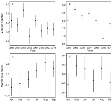
acoustic detection of harbour porpoises. A general negative trend was observed: as vessel speed increased, acoustic detection rates decreased. ‘Year’ and ‘Month’ were retained in both the visual and acoustic models. Sighting and acoustic detection rates varied among years with the highest rates occurring in 2005 (Fig. 3 a,b). Visual detections gen-erally increased with month from April to August, but then decreased in September. Two peaks in acoustic detections were observed, first in May and then again in August (Fig. 3 b,d).

Patterns of porpoise occurrence with respect to oceanographic covariates were very similar in the models built using visual and acoustic data. Seabed depth and seabed slope were the most important oceanographic covariates in both models. Porpoises were more likely to be detected in waters between 50 and 150 m (Fig. 4a,b) in depth with fewer sightings in waters < 50 or >150 m. Sighting rates increased with increasing slope up to ~10° (across 0.2 × 0.2 km grid), beyond which they decreased slightly (Fig. 4c,d). Less important oceanographic variables were also re -tained in the best models as porpoise occurrence var-ied depending on the spring tidal range (STR) e -ncountered (Fig. 4 e,f). Detections rates were highest in regions of moderate to high STR (> 4 m). Visual

and acoustic detection rates both decreased as dis-tance from land increased, with the highest rates made within 20 km of land, beyond which they decreased before increasing slightly > 30 km from land (Fig. 4 g,h). Percentage of mud was also found to impact harbour porpoise visual sighting rates, with the highest rates occurring in ∼20−60% mud.

Predicted distributions

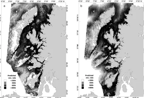
Both models predicted a strongly inshore distribu-tion for harbour porpoises throughout the west coast of Scotland (Fig. 5). The highest encounter rates were predicted in the northern Sound of Jura, northeast Firth of Lorn, within the Sound of Mull, around the Treshnish Isles to the west of Mull and throughout the Small Isles (particularly in the Sound of Sleat). Additionally, predicted rates were high along the east coast of the Outer Hebrides, throughout the Lit-tle Minch (between Skye and the Outer Hebrides) and within the more coastal reaches of the Minch. Low encounter rates were predicted in the southwest part of the study region and to the west of the Outer Hebrides islands (particularly North and South Uist).

DISCUSSION

This study illustrates that predictable, static physi-cal oceanographic features are important proxies in determining harbour porpoise distribution west of Scotland. In both visual and acoustic models, por-poise encounter rates were best predicted by seabed depth, slope, distance from land and tidal range (while sediment composition was also important in the visual model).

Harbour porpoise distribution was most heavily impacted by topographical variables (e.g. seabed depth and slope), and encounter rates were highest in regions with between 50 and 150 m water depth. A similar preference for water over 50 m depth has been recorded in other studies around the region (MacLeod et al. 2007, Goodwin & Speedie 2008, Marubini et al. 2009, Isojunno et al. 2012). Depth has also been an important predictor in other studies fur-ther afield, though the preferred depths have varied considerably (Raum-Suryan & Harvey 1998, Carretta et al. 2001, Tynan et al. 2005, Shucksmith et al. 2009). The habitat preference observed here could be explained by the availability of prey species in these regions. Major prey items for porpoises on the west coast of Scotland include juvenile whiting

Mer-Covariate df χ2 _{p Relative variable}

importance

Visual

Sea state 2 147.35 < 0.00001 −1422.5

Month 5 142.285 < 0.00001 −585.6

Year 7 84.804 < 0.00001 −511.8

Vessel speed 2 43.806 < 0.00001 −214.3

Depth 2 37.597 < 0.00001 −208.5

Slope 2 48.471 < 0.00001 −119.8

Monthly STR 4 38.234 < 0.00001 −80.7

% mud 2 79.816 < 0.00001 −71.5

Distance from land 2 20.737 0.00003 −0.3

Acoustic

Vessel speed 2 94.864 < 0.00001 −807.7

Year 6 125.399 < 0.00001 −632.7

Depth 2 69.16 < 0.00001 −490.9

Slope 4 118.338 < 0.00001 −250.5

Month 5 13.209 0.0215 −39.3

Distance from land 3 20.795 0.0001 −33.7

Monthly STR 4 50.465 < 0.00001 −28.7

Table 3. Results of Generalised Additive Models (GAM) fol-lowing model selection (with Generalised Estimating Equa-tions [GEE]) for both the visual and acoustic models. Covari-ates are ordered by their relative importance (determined by the reduction in the goodness of fit statistic QICu). If a candi-date covariate is not listed for the model, it was removed by

langius merlangus, haddock Melanogrammus aegle -finus, saithe/pollock Pollachius spp., other gadoid species, and to a lesser extent sepiolids and sandeels Hyperoplus lanceolatus(Santos et al. 2004). Fish spe-cies that tend to inhabit waters up to 200 m deep include whiting (40−200 m; Persohn et al. 2009), cod (30−200 m; Santos et al. 2004) and sandeels (30− 120 m; Wright et al. 2000) and the depth ranges they inhabit likely drive porpoise habitat use. Porpoise have also been documented feeding on a number of demersal flatfish species (Herr et al. 2009), and stud-ies of porpoise dive behaviour have shown they are capable of diving to these depths (Otani et al. 1998, Teilmann et al. 2007), indicating they are capable of feeding both demersally and pelagically for these prey species.

Seabed slope has been found to influence porpoise distribution (Bailey & Thompson 2009, Embling et al. 2010, Isojunno et al. 2012). Here, porpoise sighting and acoustic detection rates were highest in regions

with a steeply sloped seabed (although rates were low in extreme regions) (Embling et al. 2010). In contrast to our observations, porpoises have also been ob-served in areas with very shallow slopes (< 0.5°); how-ever, these observations were predominantly in deep (>125 m) waters with flat bottoms (Raum-Suryan & Harvey 1998). Little is known about the physical pro-cesses that occur in the dynamic environment of the west coast of Scotland. Generally, upwelling is a com-mon phenomenon in coastal regions of high slope as cold, nutrient-rich water is forced to the surface, in-creasing productivity and enhancing prey densities, which consequently can attract top predators (Yen et al. 2004). Slope (along with seabed friction) also drives productivity by influencing the movement of currents (Inall et al. 2009). Slope-driven upwelling is consid-ered to be temporally and spatially predictable, often centred around land features such as headlands that can serve as anchor points for eddies, rips and up-welling (Zamon 2003, Yen et al. 2004).

Fig. 3. (a,b) Year and (c,d) month relationships for the models constructed using (a,c) visual and (b,d) acoustic data, respec-tively. The relationship is shown by the point for each year/month and segments indicate the (Generalised Estimating

Fig. 4. Partial fit of each covariate from models built using (a,c,e,g) visual and (b,d,f,h) acoustic data showing the relationships (i.e.

how harbour porpoise Phocoena

phocoena detection rates fluctu-ate) with respect to: (a,b) depth, (c,d) slope, (e,f) monthly spring tidal range and (g,h) distance from land. The relationship is shown by the black line, and grey shaded areas indicate the (Generalised Estimating Equa-tion [GEE]-based) 95% confi-dence intervals. A rug plot with actual data is also shown at the base of each plot. S: smoothing

Distance to land was retained in the visual and acoustic models, and in both cases, encounter rates of porpoises generally decreased as distance from land increased. The highest predicted rates were in regions <1 to 20 km from land, indicating that the animals are exhibiting a strongly inshore distribu-tion. The uneven, fjordic coastline of the west coast means the relationship between depth and distance from land is highly variable. This covariate may be a proxy for other, unmeasured biologically significant variables. Capes and headlands can provide the anchor-points for upwelling and fronts leading to a potentially higher density of prey close to these fea-tures (Yen et al. 2004). Additionally, salinity is thought to generally decrease as distance from land increases, as the level of freshwater input is dimin-ished further offshore (Gillibrand et al. 2003). Fresh-water plume fronts (influxes of freshFresh-water meeting seawater masses) are common in inshore regions and lead to increased mixing and consequently an increase in productivity and aggregation (Yen et al. 2004).

Spring tidal range was included in both the visual and acoustic models. In both cases, a bimodal distri-bution of detection rates with respect to STR was observed with peak detection rates at 0−2 and 4−6 m. Between 2 and 4 m, significantly fewer animals were detected. STR of 0−2 m are only observed in the Sound of Jura and to the southwest of Islay while val-ues > 4 m are only observed in the waters around the Isle of Skye, in the Minch and Small Isles, indicating the inclusion of STR in the models is confounded by region.

The potential importance of seabed sediment com-position is likely a proxy for prey availability. Minke whale presence in this area has been linked to sandeel (sand/gravel) and pre-spawning herring habitat (mainly gravel) (MacLeod et al. 2004), and grey seals were observed most commonly in regions of sand and gravel which were attributed to sandeel habitats. Whiting and flatfish, which are thought to constitute the bulk of porpoise prey species around the UK (Santos et al. 2004, Herr et al. 2009), are known to prefer muddy sand sediments (Hislop 1984). Fig. 5. Predicted relative spatial patterns for the models constructed using (a) visual and (b) acoustic data displayed in

Our study shows that similar models of porpoise distribution can be generated from visual (i.e. sight-ings) and acoustic data when acoustic volumes are large. However, the automated nature of the acoustic detection makes it easier to generate a data-rich dis-tribution model and to identify important areas for the species. Acoustic detection rates were approxi-mately twice that of visual detection rates throughout the study period. Visual surveys for porpoises were most heavily impacted by sea state, with detection decreasing significantly above Beaufort sea state 1. The significant effect of vessel speed on both visual and acoustic models could be explained by animals exhibiting responsive movement, i.e. detecting and avoiding the vessel and thus decreasing detection rates (Palka & Hammond 2001). The observed pat-tern may also result from less time spent surveying in each segment at higher speeds. It is noteworthy that the patterns identified from models built using visual and towed-acoustic line transect surveys were very similar. This is interesting given that the 2 methods are subject to (some) different biases. The similarity observed here may be, in part, due to the large amounts of data available to fit the models. Studies conducted using fewer data points or more patchy effort may not be able to capture the key patterns; therefore, it is important that robust survey designs and methods be employed.

This study likely failed to capture all of the impor-tant factors involved in explaining porpoise presence in the region. The inclusion of year and month indi-cated that over the extent of the study region there were significant temporal variations in harbour por-poise sighting and acoustic detection rates. Clear annual trends were not observed in either model and detection rates fluctuated among years, suggesting that these covariates could serve as proxies for unmeasured factors that influence important vari-ables, such as prey availability or changes in detec-tion probability associated with covariates. For exam-ple, weather conditions, changes in group size and behavioural changes could all result in the animals being more or less available at the surface and/or more or less vocal, which would in turn impact sight-ings and acoustic detection rates. Both the visual and acoustic models captured similar yearly variations with peaks in 2005 and 2007. In 2009 detect ion rates were lower, but this could be accounted for by sus-pected technical issues with the PAM equipment. The peak in 2005 was previously identified by Embling (2007), who observed there was a notable change in the ecosystem of the Inner Hebrides. Minke whales had been abundant in previous years,

but their sighting rates decreased significantly in 2005. Concurrently, basking shark Cetorhinus max-imussightings increased significantly and a number of seabird species failed to fledge chicks (Stevick et al. 2007). It is currently unclear what phenomenon occurred that could exclude minke whales, whilst creating favourable conditions for porpoise and basking shark. Porpoises must maintain high daily consumption rates in order to meet their energetic requirements (Lockyer 2007) and from dietary stud-ies are known to be capable of employing a general-ist feeding strategy as their diet consgeneral-ists of many prey species (Santos et al. 2004). Therefore, it is possible that the porpoises were able to capitalise on an unex-pected shift in the ecosystem, while minke whales could not.

Seasonal variations in the models could be ex -plained either by genuine changes in harbour por-poise density and/or distribution or by changes in detection probability. Seasonal variation in harbour porpoise habitat preference and distribution in Euro-pean waters are poorly understood and have only been investigated in a handful of recent studies (e.g. Verfuß et al. 2007, Weir et al. 2007, Gilles et al. 2011). Here, we observed significant variation in detection rates between April and September. A general increase in sighting rates during summer months has been observed in other studies (Verfuß et al. 2007, Gilles et al. 2011). Peaks in sightings during the sum-mer may be indicative of better survey conditions in those months, although significant variations in sea-sonal distributions have been observed in the south-ern North Sea, indicating that animals aggregate seasonally in ‘hot spots’ within their range (Gilles et al. 2011). A different pattern was observed in the acoustic encounter rates, with peaks in detection occurring in May and August. Seasonality in por-poise vocalisations is poorly understood, but this pat-tern corresponds with the porpoise breeding season and could be explained by changes in vocal behav-iour associated with reproductive behavbehav-iour (e.g. as in Clausen et al. 2010).

Jura, Minch and Skye regions on both the mainland and east coast of the Outer Hebrides as regions with high porpoise encounter rates. The SCANS-II (2008) surveys and other modelling studies have identified the region off the west coast of Scotland to have sites suitable for designation as SACs for harbour por-poises (Marubini et al. 2009, Embling et al. 2010). Whilst the breeding behaviour of porpoises west of Scotland remains poorly understood, this study builds on this knowledge base and shows that har-bour porpoise distribution in the region is well-pre-dicted by oceanographic features, such as seabed depth and slope. Whilst there is also some temporal variation between and within years, there are key factors that can be used to identify important regions for harbour porpoises west of Scotland. Ongoing work is being conducted to investigate the long-term stability of the key regions identified here.

Acknowledgements. This work was funded under a NERC

studentship to the lead author with CASE funding from Scottish Natural Heritage. The Hebridean Whale and Dol-phin Trust were funded by the Heritage Lottery Fund, Scot-tish Natural Heritage, Argyll and the Islands Enterprise, WWF and the Earthwatch Institute. We thank all the Earth-watch and HWDT volunteers and staff who helped us to col-lect the data. In addition, great thanks to M. MacKenzie, E. Pirotta and M. Lonergan for providing statistical advice and to the reviewers for their helpful input. Thank you to all those who made covariate data available.

LITERATURE CITED

Bailey H, Thompson PM (2009) Using marine mammal habi-tat modelling to identify priority conservation zones within a marine protected area. Mar Ecol Prog Ser 378: 279−287

Bailey H, Corkrey R, Cheney B, Thompson PM (2013) Analysing temporally correlated dolphin sightings data using generalized estimating equations. Mar Mamm Sci 29: 123−141

Carretta JV, Taylor BL, Chivers SJ (2001) Abundance and

depth distribution of harbor porpoise (Phocoena

pho-coena) in northern California determined from a 1995 ship survey. Fish Bull 99: 29−39

Clausen KT, Wahlberg M, Beedholm K, DeRuiter S, Madsen PT (2010) Click communication in harbour porpoises (Phocoena phocoena). Bioacoustics 20: 1−28

CODA (2009) Cetacean offshore distribution and abun-dance in the European Atlantic (CODA). Gatty Marine Laboratory, University of St Andrews, St Andrews (avail-able online at http: //biology.st-andrews.ac.uk/coda/) Edrén SMC, Wisz MS, Teilmann J, Dietz R, Söderkvist J

(2010) Modelling spatial patterns in harbour porpoise satellite telemetry data using maximum entropy. Ecogra-phy 33: 698−708

Ellett DJ, Edwards A (1983) Oceanography and inshore hydrography of the Inner Hebrides. Proc R Soc Lond B 83B: 143−160

Embling CB (2007) Predictive models of cetacean distribu-tions off the west coast of Scotland. PhD thesis, Univer-sity of St Andrews, St Andrews

Embling CB, Gillibrand PA, Gordon J, Shrimpton J, Stevick PT, Hammond PS (2010) Using habitat models to identify suitable sites for marine protected areas for harbour

por-poises (Phocoena phocoena). Biol Conserv 143: 267−279

Evans PGH (1980) Cetaceans in British waters. Mamm Rev 10:1–52

Fox J, Monette G (1992) Generalized collinearity diagnos-tics. J Am Stat Assoc 87: 178−183

Gilles A, Adler S, Kaschner K, Scheidat M, Siebert U (2011) Modelling harbour porpoise seasonal density as a func-tion of the German Bight environment: implicafunc-tions for management. Endang Species Res 14: 157−169

Gillespie D, Chappell O (2002) An automatic system for detecting and classifying the vocalisations of harbour porpoises. Bioacoustics 13: 37−61

Gillespie D, Berggren P, Brown S, Kuklik I and others (2005)

The relative abundance of harbour porpoises (Phocoena

phocoena) from acoustic and visual surveys in German, Danish, Swedish and Polish waters during 2001 and 2002. (SC/55/SM21). J Cetacean Res Manag 7: 51−57 Gillibrand PA, Sammes PJ, Slesser G, Adam RD (2003)

Sea-sonal water column characteristics in the Little and North Minches and the Sea of Hebrides. I. Physical and Chem-ical Parameters. Fisheries Research Services, Aberdeen Goodwin L, Speedie C (2008) Relative abundance, density

and distribution of the harbour porpoise (Phocoena

pho-coena) along the west coast of the UK. J Mar Biol Assoc UK 88: 1221−1228

Halekoh U, Højsgaard S, Yan J (2006). The R package geep-ack for generalized estimating equations. J Stat Softw 15: 12−22.

Hardin JW, Hilbe JM (2002) Generalized estimating equa-tions, 2nd edn. Chapman & Hall, Boca Raton, FL Heithaus MR, Dill LM (2006) Does tiger shark predation risk

influence foraging habitat use by bottlenose dolphins at multiple spatial scales? Oikos 114: 257−264

Herr H, Fock HO, Siebert U (2009) Spatio-temporal

associa-tions between harbour porpoise Phocoena phocoenaand

specific fisheries in the German Bight. Biol Conserv 142: 2962−2972

Hislop JRG (1984) A comparison of the reproductive tactics and strategies of cod, haddock, whiting and Norway pout in the North Sea. In: Potts GW, Wootton RJ (eds) Fish reproduction: strategies and tactics. Academic Press, London

Inall M, Gillibrand P, Griffiths C, MacDougal N, Blackwell K (2009) On the oceanographic variabilty of the north-west European Shelf to the west of Scotland. J Mar Syst 77: 210−226

Isojunno S, Matthiopoulos J, Evans PGH (2012) Harbour

porpoise habitat preferences: robust spatio-temporal

inferences from opportunistic data. Mar Ecol Prog Ser 448: 155−170

Johnston DW, Westgate AJ, Read AJ (2005) Effects of fine-scale oceanographic features on the distribution and

movements of harbour porpoises Phocoena phocoenain

the Bay of Fundy. Mar Ecol Prog Ser 295: 279−293 Liang KT, Zeger SL (1986) Longitudinal data analysis using

generalized linear models. Biometrika 73: 13−22

MacLeod K, Fairbairns R, Gill A, Fairbairns B, Gordon J, Blair-Myers C, Parsons ECM (2004) Seasonal distribution

of minke whales Balaenoptera acutorostratain relation

to physiography and prey off the Isle of Mull, Scotland. Mar Ecol Prog Ser 277: 263−274

MacLeod CD, Weir CR, Pierpoint C, Harland EJ (2007) The habitat preferences of marine mammals west of Scotland (UK). J Mar Biol Assoc UK 87: 157−164

Marubini F, Gimona A, Evans PGH, Wright PJ, Pierce GJ (2009) Habitat preferences and interannual variability in

occurrence of the harbour porpoise Phocoena phocoena

off northwest Scotland. Mar Ecol Prog Ser 381: 297−310 Otani S, Naito Y, Kawamura A, Kawasaki M, Nishiwaki S, Kato A (1998) Diving behavior and performance of

har-bor porpoises, Phocoena phocoena, in Funka Bay,

Hokkaido, Japan. Mar Mamm Sci 14: 209−220

Palka D (1996) Effects of Beaufort Sea State on the sightabil-ity of harbor porpoises in the Gulf of Maine. Rep Int Whaling Comm 46: 575−582

Palka D, Hammond PS (2001) Accounting for responsive movement in line transect estimates of abundance. Can J Fish Aquat Sci 58: 777−787

Panigada S, Zanardelli M, MacKenzie M, Donovan C, Melin F, Hammond PS (2008) Modelling habitat preferences for fin whales and striped dolphins in the Pelagos Sanctuary (Western Mediterranean Sea) with physiographic and remote sensing variables. Remote Sens Environ 112: 3400−3412

Persohn C, Lorance P, Trenkel VM (2009) Habitat prefer-ence of selected demersal fish species in the Bay of Bis-cay and Celtic Sea, north-east Atlantic. Fish Oceanogr 18: 268−285

Pierpoint C (2008) Harbour porpoise (Phocoena phocoena)

foraging strategy at a high energy, near-shore site in south-west Wales, UK. J Mar Biol Assoc UK 88: 1167−1173

Pirotta E, Matthiopoulos J, MacKenzie M, Scott-Hayward L, Rendell L (2011) Modelling sperm whale habitat prefer-ence: a novel approach combining transect and follow data. Mar Ecol Prog Ser 436: 257−272

R Core Development Team (2006) R: a language and envi-ronment for statistical computing. R Foundation for Sta-tistical Computing, Vienna. www.R-project.org

Raum-Suryan KL, Harvey JT (1998) Distribution and

abun-dance of and habitat use by harbour porpoise, Phocoena

phocoena, off the northern San Juan Islands, Washing-ton. Fish Bull 96: 808−822

Read AJ, Westgate AJ (1997) Monitoring the movements of

harbour porpoises (Phocoena phocoena) with satellite

telemetry. Mar Biol 130: 315−322

Reid JB, Evans PGH, Northridge SP (2003) Atlas of cetacean distribution in north-west European waters. Report to

JNCC. Joint Nature Conservation Committee, Peters

-borough

Santos MB, Pierce GJ, Learmonth JA, Reid RJ and others

(2004) Variability in the diet of harbor porpoises (

Pho-coena phoPho-coena) in Scottish waters 1992–2003. Mar

Mamm Sci 20: 1−27

SCANS-II 2008. Small cetaceans in the European Atlantic and North Sea. Final Report to the European Commision under project LIFE04NAT/GB/000245. Sea Mammal Research Unit, Gatty Marine Laboratory, University of St Andrews, St Andrews

Scheidat M, Verdaat H, Aarts G (2012) Using aerial surveys to estimate density and distribution of harbour porpoises in Dutch waters. J Sea Res 69: 1−7

Shucksmith R, Jones NH, Stoyle GW, Davies A, Dicks EF (2009) Abundance and distribution of the harbour

por-poise (Phocoena phocoena) on the north coast of

Angle-sey, Wales, UK. J Mar Biol Assoc UK 89: 1051−1058 Stevick PT, Calderan SV, Speedie C, Shrimpton J, Embling

CB (2007) A trophic shift off West Scotland: minke

whales and basking sharks. 21st Annual Conference of the European Cetacean Society, San Sebastian

Sveegaard S, Teilmann J, Berggren P, Mouritsen KN, Gille-spie D, Tougaard J (2011) Acoustic surveys confirm areas of high harbour porpoise density found by satellite track-ing. ICES J Mar Sci 68: 929−936

Sveegaard S, Nabe-Neilsen J, Staehr KJ, Jensen TF, Mourit-sen KN, Teilmann J (2012a) Spatial interactions between marine predators and their prey: herring abundance as a driver for the distributions of mackerel and harbour por-poise. Mar Ecol Prog Ser 468: 245−253

Sveegaard S, Andreasen H, Mouritsen KN, Jeppesen JP, Teilmann J, Kinze CC (2012b) Correlation between the seasonal distribution of harbour porpoises and their prey in the Sound, Baltic Sea. Mar Biol 159: 1029−1037 Swift RJ, Caillat M, Gillespie D (2008) Appendix D2.3:

analysis of acoustic data from SCANS-II survey. In: SCANS-II. Small cetaceans in the European Atlantic and North Sea. Final Report to the European Commission under project LIFE04NAT/GB/000245. Sea Mammal Research Unit, Gatty Marine Laboratory, University of St Andrews, St Andrews, p 55

Teilmann J (2003) Influence of sea state on density estimates

of harbour porpoises (Phocoena phocoena). J Cetacean

Res Manag 5: 85−92

Teilmann J, Larsen F, Desportes G (2007) Time allocation

and diving behaviour of harbour porpoises (Phocoena

phocoena) in Danish and adjacent waters. J Cetacean

Res Manag 9: 201−210

Tynan CT, Ainley DG, Barth JA, Cowles TJ, Pierce SD, Spear LB (2005) Cetacean distributions relative to ocean processes in the northern California Current System. Deep-Sea Res II 52: 145−167

Verfuß UK, Honnef CG, Meding A, Dahne M, Mundry R, Benke H (2007) Geographical and seasonal variation of

harbour porpoise (Phocoena phocoena)presence in the

German Baltic Sea revealed by passive acoustic monitor-ing. J Mar Biol Assoc UK 87: 165−176

Weir CR, Stockin KA, Pierce GJ (2007) Spatial and temporal trends in the distribution of harbour porpoises, white-beaked dolphins and minke whales off Aberdeenshire (UK), north-western North Sea. J Mar Biol Assoc UK 87: 327−338

Wright PJ, Jensen H, Tuck I (2000) The influence of sedi-ment type on the distribution of the lesser sandeel,

Ammodytes marinus.J Sea Res 44: 243−256

Yen PPW, Sydeman WJ, Hyrenbach KD (2004) Marine bird and cetacean associations with bathymetric habitats and

shallow-water topographies: implications for trophic

transfer and conservation. J Mar Syst 50: 79−99

Zamon JE (2003) Mixed species aggregations feeding upon herring and sandlance schools in a nearshore archipel-ago depend on flooding tidal currents. Mar Ecol Prog Ser 261: 243−255

Editorial responsibility: Peter Corkeron, Woods Hole, Massachusetts, USA

Submitted: July 2, 2012; Accepted: December 27, 2012 Proofs received from author(s): March 11, 2013