Greedy and linear ensembles of machine learning methods outperform single approaches for QSPR regression problems

Greedy and Linear Ensembles of Machine Learning Methods

Outperform Single Approaches for QSPR Regression Problems

William Kew

and John BO Mitchell

Biomedical Sciences Research Complex and EaStCHEM School of Chemistry, Purdie Building, University of St Andrews, North Haugh, St Andrews,

Scotland, KY16 9ST, UK

* Corresponding author: email [email protected]

†

A

BSTRACT

The application of Machine Learning to cheminformatics is a large and active field of research, but there exist few papers which discuss whether ensembles of different Machine Learning methods can improve upon the performance of their component methodologies. Here we investigated a variety of methods, including kernel-based, tree, linear, neural networks, and both greedy and linear ensemble methods. These were all tested against a standardised

methodology for regression with data relevant to the pharmaceutical development process. This investigation focused on QSPR problems within drug-like chemical space. We aimed to

investigate which methods perform best, and how the ‘wisdom of crowds’ principle can be applied to ensemble predictors. It was found that no single method performs best for all problems, but that a dynamic, well-structured ensemble predictor would perform very well across the board, usually providing an improvement in performance over the best single method. Its use of weighting factors allows the greedy ensemble to acquire a bigger

1 I

NTRODUCTION

Cheminformatics relies on informatics, statistical and Machine Learning (ML) methodology, rather than directly modelling the physics of the real world, to study chemical and biochemical systems.[1] Cheminformatics can address diverse problems in chemistry, from molecular docking to quantitative structure-activity relationships (QSAR), and can be used to improve the quality of experimentally obtained data, for example by reducing noise in high-throughput screening data.[2] One of the most significant areas of application for cheminformatics techniques is in medicinal chemistry and drug development.[3,4,5,6,7]

QSAR is based on the principles that the physiochemical properties of a molecule are related to its structure, and that similar structures tend to exhibit similar properties. The principles of QSAR can be expanded to include wider contexts of application, such as quantitative structure-property relationships (QSPR), or similarly for selectivity (QSSR) or toxicity (QSTR).

While the basic principles underlying a QSAR relationship can often be rationalised in a general chemical sense – such as the presence of a polar group in a molecule making it more soluble in a polar solvent, QSARs are empirical in nature. The field has moved on from simple linear and multi-linear regression, and more complex relationships require more complex determination, and this is where ML comes in. It is also worth remembering that correlation does not equal causation, and most ML and cheminformatics methods do not, and cannot, determine causation.

Machine Learning is a field of artificial intelligence which concerns the ability to train a

computer system, using existing data, to be able to predict properties of new, unseen, data. This has become increasingly important in recent years given both the huge growth in computing power and the exponential advance of Big Data..[1] Technical developments within computer science have allowed ML to infiltrate many aspects of modern life in a wide variety of

applications. These can include, but are by no means limited to, cheminformatics,[8] as well as the closely related field of bioinformatics,[9,10,11] image processing,[12]text analysis,[13] and even learning to play video games.[14,15] As Helfert et al. observed, “Data can be a mixed

blessing…”,[16]and this can certainly be true with the expanse of Big Data. However, with the power of sophisticated computers and algorithms,[17] _{ML allows problems to be addressed in}

modern and powerful ways. Machine Learning, in the context of cheminformatics and QSAR, often involves an overarching workflow of dataset construction, training and optimising models, and then testing them on new data.

Most cheminformatics investigations tend to focus on one or a small number of ML methods and only one or two chemical problems.[18,19,20,21] Here, we look at a large number of ML

methods and compare them on a standard methodology across a number of datasets of varying size and properties, to examine which methods perform best. Further, we consider ensemble ML methods, which are under-represented in the literature. The aim was to see how these can be developed and utilised in diverse cheminformatics problems, and if they indeed perform in accordance with the ‘wisdom of crowds’[8,22,23]principle; that if a single prediction is good, many predictions - averaged in some way - are better.

excretion and bioavailability.[24] Since aqueous solubilities can have a very large range, we quote and predict them as the base 10 logarithm, logS, where S is referred to molar units. It was known as early as 1924[25] that aqueous solubility is, at least somewhat, predictable from chemical structure – in that case by comparing the number of methyl groups on otherwise similar molecules, with aqueous solubility being related to molecular size. Much further work has been done, and various other properties have been shown to relate, including the melting point and octanol-water partition coefficient as exemplified in the General Solubility Equation and elsewhere.[20,24,26]Much of the solubility data used here came from the Solubility

Challenge,[27,28] a competition to challenge research groups to develop and test computational means of accurately predicting solubility. These data were obtained in one laboratory by a standardised and sophisticated experimental procedure, CheqSol.[29] That being said, all experimental data have some associated error, and quality of data is crucial in ML. Indeed, our recent study has shown that, despite its apparently small random error, use of data exclusively from CheqSol is not a panacea for all difficulties in modelling solubility.[30] For a typically difficult set of druglike molecules, it is reasonable to suggest that computing their logS values to within a ±1 logS unit root mean squared error (RMSE) is a good prediction.[31]

The octanol-water partition coefficient is important for ensuring bioavailability in drug development,[32] and allowing the drug to cross membranes as required.[20,24]It is generally regarded as a measure of lipophilicity. Like aqueous solubility, the partition coefficient is quoted as its base 10 logarithm, logP, due its potentially large range of values. The ability to quickly and easily predict logP in silico is very useful to the wider community, given the large reliance on focusing on potency of compounds, rather than ADMET optimisation in drug development.[32] LogP values are known from previous work, including our own, to be easier to predict than logS values; [24]nonetheless, there is scope for considerable improvement upon currently available methods.

Melting point is also important in drug development,[24] though perhaps less obviously so. For example, if one could predict the melting point of a novel compound accurately, it might aid in the characterisation of that substance. Melting point also plays a key role in the General Solubility Equation.[26] Whilst melting points have shown some predictability in the

literature[18,19,21,24,33]they are notoriously difficult to compute accurately – this is argued to be due to a relationship to 3D structure and bulk properties not adequately described by 2D descriptors of single molecules.[24] Based on literature and prior work in our group, a

predictability of ±50°C in terms of RMSE (reference[18]uses the more forgiving “average absolute error” measure) might be considered reasonable.[18,19,21,24,33]

2 M

ETHODS

2.1 ALGORITHMS

2.1 General Linear Model

The first of three simple, and similar, linear methods we have investigated is the General Linear Model (GLM),[34] a simplistic multivariable model based on linear regression, not dissimilar to simply plotting X versus Y and extrapolating. It is susceptible to various sources of error, including over-fitting, and we did not expect it to perform very well on complex problems. It is used here for constructing a simple linear ensemble, and is called with the keyword glm in the statistical programming suite R.[35]

2.1.2 Partial Least Squares

Partial Least Squares (PLS) is a long standing technique in modelling, traced back to the 1960’s, and initially used in economics.[36] In wider chemistry applications, PLS can be used for

calibration of spectrometers. It is an advanced evolution of multiple linear regression, and attempts linear regression for a system with many collinear variables by reducing the number of variables to those which are most significant for predicting the outcome. It is a relatively cheap and simple method, which may not perform very well on complex problems. In the R scripts, it is called using the pls keyword.

2.1.3 Principal Components Regression

Closely related is Principal Components Regression (PCR), a method which builds a linear regression model based on the principal components.[36] Given that Principal Component Analysis (PCA) is used as one of the pre-processing methods in this work, PCR is of limited significance to us here. In the R scripts used here, it is called with the pcr keyword.

2.1.4 K-Nearest Neighbours

One of the easiest methods to understand in ML is k-nearest neighbours (kNN), an approach used somewhat commonly for QSAR and related problems.[37,38] It is based on the assumption that molecules close together in descriptor space will have similar properties.[8] kNN will simply predict a test molecule as having the same properties as its nearest neighbour (within the training set) when k=1, but with k>1 kNN regression’s output prediction is based on an average of the neighbours’ properties. kNN is used here via the knn keyword in R.

2.1.5 Neural Networks

2.1.6 Tree Methods (Random Forest, Treebag and Cubist)

Another relatively easy family of algorithms to understand are the tree-based methods. In the simplest form, these consist of simple decision trees – like flowcharts – constructed from the training data. One of the most effectively and commonly[43] used ways to improve upon the simple decision tree is to use Random Forest (RF), an ensemble technique wherein a large number of trees are constructed, hence forest,[44,45] and their outputs are combined to produce a consensus result. The ensemble method here trains the forest to produce diverse trees by giving each tree a different subset of the descriptors to learn from. In this investigation 1000 trees were used, as the additional computational cost was negligible, though it is generally considered that around 500 trees are sufficient to obtain the full benefit of the ‘wisdom of crowds’ consensus effect.[43] The Random Forests were implemented with the rf keyword in R. Another tree based ensemble method, related to Random Forests, was also used – treebag. This bagged (bootstrap aggregation) method is produced in a similar fashion to Random Forests, except each tree is this time trained on a reduced subset of the available input training data.[43] Though this approach predates Random Forest, it is no longer as popular since it is considered less sophisticated. Finally, and slightly differently, cubist is a rule-based regression method,[46] developed in the late 1990’s, and has had limited coverage in the literature given its proprietary origins. However, an R port based on GPL code released by the developers was developed by Kuhn,[47] where a tree is grown as normal, but the decisions are reduced to a set of rules, by pruning amongst other methods. This method has not been investigated widely in

cheminformatics, and this work provides an interesting opportunity to benchmark the performance of a relatively underexposed technique.

2.1.7 Kernel-Based Methods (Support Vector Machine, Relevance Vector Machine and Gaussian Processes)

One of the more widely used methods used in this field these days is Support Vector Machine (SVM). This method takes the data, maps them in a high-dimensional feature space, and attempts to plot a hyperplane separating two classes by maximising the distance between the plane and the support vectors, or closest points in space.[8,48] Particular mathematical functions – kernels - are used to enable linear classification, as well as numerical regression on non-linear data. SVM is therefore used as a kernel-based regression method in this investigation. SVM is called with the keyword SVM followed by the kernel function suffix. Two kernel functions were used here; radial, and polynomial. The linear kernel, despite being a less computationally expensive function, was not included since it performed poorly in preliminary work. The radial kernel has previously been investigated in our laboratory,[31] and indeed has proven quite successful for a variety of cheminformatics problems.[8,49,50,51] The polynomial kernel function is by far the more expensive kernel function of those considered here. As such, less parameter optimisation was conducted for polynomial methods than radial ones. The two kernels are defined with the R keyword suffixes of Radial, and Poly, respectively. In addition to SVM, two other kernel-based methods were used. The first of these was Relevance Vector Machine (RVM). Otherwise very similar to SVM, RVM uses Bayes’ theorem and an assumed Bernoulli distribution of conditional probabilities to output probabilistic classification and regression models.[52] RVM, in favourable cases at least, has comparable performance at reduced

investigation is for the comparison of kernel methods. It was used with the R keyword prefix gaussPr.

2.1.8 Ensemble Methods (Greedy Ensemble and Linear Ensemble)

One of our main aims here is to develop a methodology with ensemble methods, and

investigate their performance. To that end, the recently developed caretEnsemble package[56] was utilised to build two further models. Once each of the previously mentioned models had been trained, these additional ensemble, or consensus, models were generated from them. Ensemble models were constructed in two different ways – a greedy ensemble

(ens_greedy),[57,58] and a simple linear stacked ensemble (ens_linear). The linear ensemble simply used a further glm model to combine the other models into one ensemble. This method is inherently susceptible to error if one or more of the constituent models is performing badly. The greedy ensemble takes a weighted amount of the best-performing constituent models based on their performance within an internal validation set. It is based upon greedy algorithms, which attempt to find an optimal solution to a problem. These are not perfect, and may fail to consider all possibilities.[57] The exact weightings chosen will vary with each fold of each dataset, and so this dynamic nature means the greedy ensemble can be tuned to perform well for each problem. Thus we obtain a dynamically generated ensemble that does not require hardcoding of methods into or out of the model depending on their individual effectiveness, but instead automatically fine tunes their weights. The Random Forest and treebag methods, discussed earlier, are technically themselves ensemble methods also, although with their constituent parts being tree-based.

2.2 S

OFTWARE

U

SED

2.2.1 R

R (version 3.0.2)[35]– a programming language and computer environment for statistics – was chosen for its relative ease of use as well as its diverse set of plugins and abilities, due to its scripted nature. Within R, various plugins – known as packages – were used here to expand the list of available ML algorithms, as well as to provide ways to optimise these methods. These packages include Kernlab,[59]Metrics,[60]randomForest,[61] and several others. The main

functions of the script were provided by the caret[62] package, which acts as a wrapper for many ML methods, unifying syntax and simplifying development and scaling of the script. The

ensemble methods, discussed above, were implemented with an extension to the caret package, the caretEnsemble[56] package.

2.2.2 CDK Descriptor Calculator

For calculation of descriptors, we used the CDK Descriptor Calculator GUI, CDKDescUI[63](version 1.4.1). This software takes a comma-delimited list of compounds (in SMILES format) and

calculates over 200 descriptors. For this methodology, all possible descriptors were calculated for each molecule. Descriptors which returned an N/A were removed, as well descriptors which showed zero, or near-zero variance (based on the nearZeroVar function in the caret package in R). The descriptors were then further pre-processed in two different ways, either with simple centre-scaling (CS) to normalise divergent numbers, or with Principal Component Analysis (PCA) to reduce the descriptors to a lesser number of principal components. The PCA functionality was implemented using the pre-processing function of the caret package. Exact numbers of

2.2.3 Taverna

A Taverna workflow was used to convert chemical names to their corresponding SMILES strings, required for descriptor calculation. This workflow[31] queried the Chemspider online database.[64]

2.2.4 Experimental Design

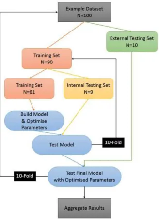
The methodology of the R script is demonstrated in Figure 1. This represents the workflow of the process. For a given dataset with N=100 molecules, the dataset is split into a training set and a test set. This external dataset of 10% of the total data is withheld from all training, meaning that the results from testing on the final model are valid, and not based on examples that the trained models have previously seen. This important aspect is discussed widely in the

literature.[8,65, 66]

The training set is then split again 90-10 for training and internal validation. This internal validation set is used for cross-fold validation to make sure that the final trained model is not biased on one split of the data. The sections of the flowchart in blue represent what the caret package in R can do. That is, it will run the ML methods several times to determine the optimum parameters – e.g., the size of a neural network, or the number of k-nearest neighbours to use. It determines this by scoring the methods against this internal validation set. Additionally, these scores are used by the caretEnsemble package to determine weightings for the greedy ensemble method.

The final model, once trained on the complete training set, including parameter optimisation with the internal validation set, is then scored against the external testing set. This score is aggregated across a 10-fold cross-validation to provide a real measure of the performance. Averaging over splitting the dataset in 10 different random ways gives a fair measure; here, the process was also repeated five times with different random seeds, given in the scripts in the SI.

2.3 M

EASURING

P

ERFORMANCE

2.3.1 RMSE

For simple numerical regression, Root-Mean-Square Error (RMSE) is commonly quoted, and for a dataset with positive and negative numbers, it provides a real comparison of predicted versus actual values. In this investigation, the RMSE was calculated for each method, for each fold, and then averaged across the entire process, including with five different random seeds. The RMSE value is given in the appropriate units of the given problem, for example logS units for solubility.

2.3.2 Normalised RMSE

When comparing different datasets, especially for different problems – solubility and melting points, for example – the RMSE values are no longer directly comparable. Thus, in addition to RMSE, we also calculated Normalised RMSE values – whereby the RMSE value was divided by the range of actual values of each experimental property in the dataset.

2.3.3 R

melting point), stripping out systematic bias. The latter will affect our RMSE, but not R2, values.

Figure 1 – Schematic flowchart of our methodology. This tenfold cross-validation process is repeated five times with five different random seeds for each combination of algorithm and dataset.

2.3.4 Alternative Approaches

margin might be within 0.5 logS units of experiment, as in the solubility challenge,[27,28] or perhaps 1.0 logS unit; experimental errors have been estimated to be around 0.6-0.7 logS units.[68]Any prediction falling within the specified range would be considered valid. In previous investigations[31] this has been used as a metric, however it is not discussed further here.

3 R

ESULTS

3.1 Aqueous Solubility (logS)

The first problem investigated was that of predicting aqueous solubility, logS, of compounds. This built on prior work by the Mitchell group, and indeed the initial dataset was taken from this work,[31] and shall be referred to as the ‘Solubility Challenge’ (SC) dataset in this paper; it

represents the usable subset of the original SC data.[27,28, 31]

A second dataset for this chemical problem allows comparison of dataset size and quality, keeping methods constant, allowing for greater analysis of results. This second dataset was taken from previous work within the Mitchell group, [24] and shall be referred to as the ‘Laura Hughes’ dataset, abbreviated to ‘LH’ dataset, for the rest of this paper. Importantly, the LH data also have available values for logP and melting point, which facilitate comparison between the predictions of different physicochemical properties.

Descriptors for both datasets were calculated in the same way, with the same CDK software.[63]

Dataset Molecules Descriptors

Solubility Challenge 122 113

Laura Hughes 262 139

Table 1: Datasets for logS models

Table 1 shows the different sizes of the two logS datasets. Whilst they cover the same regions of chemical space, the LH dataset is more than twice the size of the SC dataset, and therefore should produce better models for predicting logS. The difference in number of descriptors is not hugely significant – the LH dataset has more descriptors because it has more molecules, and therefore fewer calculated descriptors will have had zero variance or near zero variance.

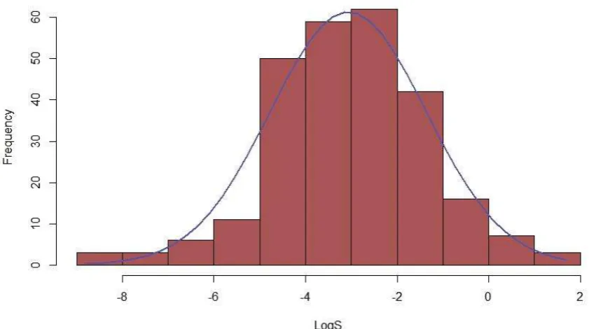
Figure 2 - Histogram of logS distribution for the Solubility Challenge dataset

RMSE RVM Radial RVM Poly SVM Radial SVM Poly GaussPr Radial GaussPr Poly

nnet kNN treebag RF cubist PLS PCR ens

greedy ens linear

SC (PCA) 1.12 0.92 0.96 0.95 1.03 0.94 1.09 0.98 1.06 1.03 0.90 0.91 0.88 0.84 0.85

SC (CS) 1.21 0.91 0.94 0.91 0.96 0.88 1.07 0.95 0.94 0.89 0.86 0.93 0.92 0.83 0.86

LH (PCA) 1.26 1.19 1.08 1.15 1.17 1.20 1.21 1.19 1.20 1.15 1.17 1.20 1.19 1.09 1.17

LH (CS) 1.22 1.22 1.01 1.07 1.03 1.10 1.38 1.15 1.05 1.02 1.09 1.14 1.12 1.03 1.08

Norm RMSE RVM Radial RVM Poly SVM Radial SVM Poly GaussPr Radial GaussPr Poly

nnet kNN treebag RF cubist PLS PCR ens

greedy ens linear

SC (PCA) 0.16 0.13 0.14 0.13 0.15 0.13 0.15 0.14 0.15 0.14 0.13 0.13 0.12 0.12 0.12

SC (CS) 0.17 0.13 0.13 0.13 0.14 0.12 0.15 0.13 0.13 0.12 0.12 0.13 0.13 0.12 0.12

LH (PCA) 0.12 0.11 0.10 0.11 0.11 0.11 0.12 0.11 0.11 0.11 0.11 0.11 0.11 0.10 0.11

LH (CS) 0.12 0.12 0.10 0.10 0.10 0.10 0.13 0.11 0.10 0.10 0.10 0.11 0.11 0.10 0.10

R2 RVM

Radial RVM Poly SVM Radial SVM Poly GaussPr Radial GaussPr Poly

nnet kNN treebag RF cubist PLS PCR ens

greedy ens linear

SC (PCA) 0.46 0.57 0.53 0.55 0.56 0.56 0.45 0.51 0.44 0.47 0.58 0.56 0.58 0.63 0.62

SC (CS) 0.42 0.56 0.54 0.57 0.55 0.58 0.48 0.54 0.55 0.60 0.60 0.54 0.55 0.63 0.61

LH (PCA) 0.48 0.56 0.59 0.57 0.59 0.54 0.52 0.52 0.53 0.55 0.56 0.54 0.54 0.60 0.56

LH (CS) 0.51 0.58 0.64 0.61 0.64 0.59 0.39 0.53 0.61 0.63 0.60 0.57 0.57 0.63 0.60

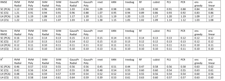
The RMSE values for aqueous solubility are shown in the top panel of Table 2. For the SC dataset, the RMSE values are encouragingly mostly within 1 logS unit. Nonetheless, some models produced much lower (better) RMSE values than others. For the dataset with simple CS pre-processing, the range of results was 0.83-1.21 logS units. The best method was the greedy ensemble, with an RMSE of 0.83. The linear ensemble performed almost as well with an RMSE of 0.86. Looking at the more traditional methods, it is clear that the kernel based methods (RVM, SVM, and Gaussian Processes) perform better with a polynomial kernel function,

especially the RVM which had an error of 1.21 logS units with the radial function and 0.91 with the polynomial function, a significant performance boost from the latter kernel. In this instance, the best kernel-based method was Gaussian Processes with the polynomial function, at 0.88 logS units. Of the tree and rule based methods, cubist outperforms treebag and Random Forests with an RMS error of 0.86 – equally good as the linear ensemble. The simple, fast, linear

methods – PLS and PCR – performed reasonably well in this case too. The greedy ensemble scored better than any of the individual models it was comprised of, as expected from the ‘wisdom of crowds’ hypothesis.

The SC dataset was also modelled with PCA pre-processing. This reduced the computational cost significantly, cutting the time to train and test models by over half. This came at the cost of slightly worse predictivity for most models; the range of RMSEs recorded was smaller, but with a slightly larger minimum RMSE, at 0.84-1.12. Again the greedy and linear ensembles performed very well, with both doing better than any of their constituent models. The kernel methods again performed better with the larger polynomial function than with the radial function, but the performance difference is not as great as for the CS pre-processing. Neural networks had an RMSE of 1.09 here, compared with 1.07 RMSE for CS pre-processing, a minimal difference, but notably worse than most of the other ML methods. Again the cubist method performed better than treebag or Random Forest, but less well than it did with CS pre-processing. Only three models performed better with PCA than CS pre-processing – RVM with a radial kernel function, PLS and PCR. Possibly these methods are more sensitive to descriptor noise, and would benefit more from more thorough dataset curation and pre-processing.

The R2values, in Table 2, support similar conclusions to the RMSE analysis. For Solubility

Challenge data with CS pre-processing, only two models had R2 below 0.5 – neural networks and RVM with the radial kernel function. However, with PCA pre-processing this benchmark was missed by two more methods, treebag and Random Forests. Again, greedy and linear ensembles outperformed their constituent models, with the greedy achieving an R2 of 0.63 for both pre-processing methods. It is clear that many of the methods perform essentially equally well.

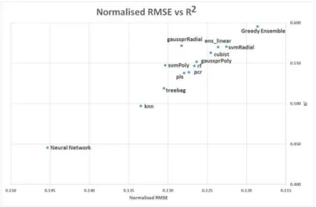
The ranges of RMSEs for the LH dataset are larger than for SC, at 1.01-1.38 and 1.09-1.26 for CS and PCA pre-processing, respectively. When we normalised the RMSE values, see middle panel of Table 2, the LH dataset was actually modelled better in relative terms. This demonstrates the importance of normalising measures when comparing different datasets. As shown in the LH dataset histogram, Figure 3, the range of logS values was greater than for the SC dataset. Therefore the RMSE scores for the LH data were normalised from a wider range onto the standardised scale, and proportionally scored better, see Figure 4.

methods, the radial function usually out-performed the polynomial kernel. This is in direct contrast to the SC dataset. Also unlike the SC dataset, random forests performed best of the tree-based methods – better than cubist or treebag. The worst model was the neural network, with a poor RMSE of 1.38. These trends were generally mirrored with PCA pre-processing, albeit it with poorer RMSE values for most of the models. Two models did perform better with PCA than with simple CS pre-processing, RVM with the polynomial function and neural networks. Again, this is different to the SC dataset. Neural networks may favour the PCA pre-processing as it reduces noise in the data, and therefore prevents overfitting.[8]

The R2values for the LH logS dataset are shown in the lower panel of Table 2 and in Figure 4. For CS, the joint best R2values were for SVM and Gaussian Processes with the radial kernel – both obtaining 0.64, which is higher than for the SC dataset. The greedy ensemble had R2 = 0.63 with CS scaling, matching the SC dataset, but with PCA its R2 dropped to 0.60. Two models failed to reach an R2value of greater than 0.5, neural networks with CS pre-processing and RVM radial with PCA. With the alternative pre-processing protocols, both methods built models with R2 above 0.5.

3.2 Octanol-Water Partition Coefficient (logP)

The second chemical problem investigated was predicting the base 10 logarithm of the octanol-water partition coefficient, logP, for which values were available in the LH dataset. [24]

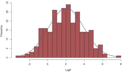
Figure 5 shows the distribution of logP values within the LH dataset, with the numbers of molecules and descriptors being as detailed in Table 1. This histogram most closely resembles a Gaussian distribution. There are outliers at very high and low logP, but the majority are within the range associated with Lipinski drug like space, with a logP of less than 5

[69,70] _{Based on prior work in the literature, and with this dataset, logP was expected to be the}

easiest numerical regression problem to model.

Figure 5 - Histogram of logP distribution for the Laura Hughes dataset.

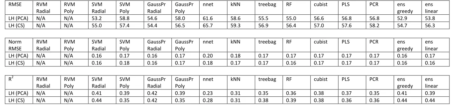
Table 3 also shows the R2 values for the logP models. For the partition coefficient problem, the R2values were all substantially higher than for logS, with the lowest value being 0.54 for neural networks with the CS pre-processing. The analysis of R2 values supports the RMSE conclusions, the greedy ensemble performing very well again with values of 0.73 and 0.70 for CS and PCA, respectively. For CS, other models which scored highly include SVM radial, Gaussian Processes polynomial, random forests and cubist, each with an R2of 0.72 or 0.73. In contrast, however, the highest R2value for PCA pre-processed models was Gaussian processes with a radial function, obtaining a value of 0.71 – interestingly this was higher than the R2 obtained by either the greedy or linear ensembles.

3.3 Melting Points

The final regression problem investigated was that of predicting the melting points of

RMSE RVM Radial RVM Poly SVM Radial SVM Poly GaussPr Radial GaussPr Poly

nnet kNN treebag RF cubist PLS PCR ens

greedy ens linear

LH (PCA) 1.11 1.08 1.06 1.15 1.16 1.07 1.09 1.18 1.23 1.18 1.07 1.08 1.10 1.04 1.14

LH (CS) 1.15 1.20 1.01 1.25 1.11 1.04 1.40 1.21 1.07 1.02 1.01 1.08 1.08 1.01 1.07

Norm RMSE RVM Radial RVM Poly SVM Radial SVM Poly GaussPr Radial GaussPr Poly

nnet kNN treebag RF cubist PLS PCR ens

greedy ens linear LH (PCA) 0.10 0.10 0.10 0.11 0.11 0.10 0.10 0.11 0.11 0.11 0.10 0.10 0.10 0.10 0.11 LH (CS) 0.11 0.11 0.09 0.12 0.10 0.10 0.13 0.11 0.10 0.09 0.09 0.10 0.10 0.09 0.10

R2 RVM

Radial RVM Poly SVM Radial SVM Poly GaussPr Radial GaussPr Poly

nnet kNN treebag RF cubist PLS PCR ens

greedy ens linear

LH (PCA) 0.67 0.68 0.69 0.65 0.71 0.69 0.67 0.64 0.59 0.64 0.69 0.68 0.67 0.70 0.66

LH (CS) 0.65 0.69 0.73 0.68 0.70 0.72 0.54 0.62 0.70 0.73 0.72 0.69 0.69 0.73 0.70

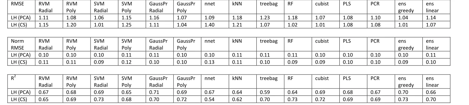
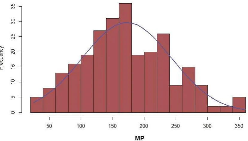
RVM methods failed to run successfully in R for the melting point models. As such they were removed from the script for melting point modelling, and are not constituents of the greedy or linear ensembles for these models. Table 4 shows that again the greedy ensemble performed best, with RMSEs of 54.7°C and 52.9°C for CS and PCA pre-processing, respectively. Whilst this size of RMSE is in line with the literature, being over 50°C out for a melting point prediction is a significant error and limits the usefulness of the models, especially when, as shown in Figure 6, the spread of melting points is only around 350°C in total. Again the ‘wisdom of crowds’ principle is obeyed, with the greedy ensemble doing better than any of its constituent models. Of the kernel-based methods, SVM with the radial function performs best with PCA with an RMSE of 53.2°C, and Gaussian Processes with the radial kernel perform best with CS, having an RMSE of 54.4°C. Consistent with the logS and logP regression problems, neural networks perform worst for both CS and PCA pre-processing, with RMSEs of 65.7°C and 61.6°C, respectively.

Unlike the other regression problems, it appears that more models were improved with PCA compared with CS pre-processing. Indeed only SVM with the polynomial function, and Gaussian Processes with the radial function, performed better with CS than PCA. Of the tree based methods, cubist performed worst, with treebag and Random Forests doing approximately equally well.

As seen in Table 4, the R2values across the board are low. The highest R2 is 0.44, achieved by both SVM radial and the greedy ensemble with PCA pre-processing. Neural networks obtained a disappointing R2 of 0.23 with CS processing, only slightly improving to 0.28 with PCA pre-processing. Generally the trends in R2mirrored those of RMSE. PCA pre-processing did better than CS for most melting point models. The greedy ensemble did well, while again neural

networks performed poorly, especially in terms of R2. Finally, as expected, melting points proved the most difficult of the three properties to model, as evidenced by the larger normalised RMSE and the smaller R2 values.

3.3 Comparison across the three problems

Table 5 shows the averaged normalised RMSE and R2 _{values across the three problems for a}

RMSE RVM Radial RVM Poly SVM Radial SVM Poly GaussPr Radial GaussPr Poly

nnet kNN treebag RF cubist PLS PCR ens

greedy ens linear

LH (PCA) N/A N/A 53.2 58.8 54.6 58.0 61.6 58.6 55.5 55.0 56.6 56.8 56.8 52.9 53.8

LH (CS) N/A N/A 55.0 57.4 54.4 56.5 65.7 59.3 56.9 56.4 57.0 57.6 58.2 54.7 56.3

Norm RMSE RVM Radial RVM Poly SVM Radial SVM Poly GaussPr Radial GaussPr Poly

nnet kNN treebag RF cubist PLS PCR ens

greedy ens linear LH (PCA) N/A N/A 0.16 0.17 0.16 0.17 0.20 0.18 0.17 0.17 0.17 0.17 0.17 0.16 0.17 LH (CS) N/A N/A 0.16 0.18 0.16 0.17 0.18 0.17 0.17 0.16 0.17 0.17 0.17 0.16 0.16

R2 RVM

Radial RVM Poly SVM Radial SVM Poly GaussPr Radial GaussPr Poly

nnet kNN treebag RF cubist PLS PCR ens

greedy ens linear

LH (PCA) N/A N/A 0.41 0.39 0.42 0.39 0.23 0.31 0.35 0.36 0.38 0.37 0.35 0.41 0.39

LH (CS) N/A N/A 0.44 0.35 0.42 0.35 0.28 0.31 0.38 0.39 0.38 0.36 0.36 0.44 0.44

Table 4: Results of regression models for melting point using the various ML methods showing (top) RMS errors in °C; (middle) normalised RMS errors, see text for details; (bottom)

Figure 6 - Histogram of melting point distribution for the Laura Hughes dataset.

Average SVM Radial

Gausspr Poly

nnet cubist PLS ens

greedy

ens linear

NRMSE 0.12 0.13 0.15 0.12 0.13 0.12 0.12

R2 0.57 0.55 0.45 0.56 0.54 0.60 0.57

4 D

ISCUSSION

Across the three related chemical regression problems, 15 different ML methods were directly compared. A summary of their performance is presented in Figure 4 and Tables 2, 3, 4, and 5. Looking at the average normalised RMSE and R2values, the best models were the greedy ensemble, RVM polynomial (when it worked), SVM radial, and cubist. The greedy ensemble, a dynamically generated ensemble of up to 13 models, managed to consistently do as well as, or better than, any of its constituent models, with the linear ensemble slightly behind it. The similar linear model was more susceptible to errors from poor component models, and thus did not perform as well. With careful model selection, it would be probably possible to train a linear ensemble to perform much better. Random Forests, itself an ensemble method but comprising only regression trees, also produced reasonable models. As shown in the lower panels of Tables 2, 3 and 4, average R2values for each method with either PCA or CS pre-processing demonstrate how some methods are more suited to one of the other, or have no preference. This is most noticeable with neural networks, which averaged an R2of 0.41 with CS, but improved to 0.48 with PCA. The most significant opposite trend was for Gaussian Processes with a polynomial kernel, which achieved an average R2for 0.57 with CS, but only 0.54 with PCA.

Given that aqueous solubility is widely considered to be difficult to model and predict, 20,24, 27,31,69

the RMSE and Rvalues obtained here for solubility prediction were reasonably good. Previous work with the LH dataset24 did obtain better predictivity, however the experimental design and methodology were different in that investigation. The availability of two different datasets, of different sizes, provided an interesting comparison. Overall ensemble methods performed well for solubility, whether they were Random Forests or greedy (or linear) ensembles mixing different ML methods.

Overall trends which can be drawn from our logP modelling include that, again, ensemble methods perform well. The linear ensemble does not perform as successfully as the greedy ensemble, but this is probably due to its indiscriminate formation from all models, some of which – e.g., neural networks – don’t perform well. Again cubist performs well, as do random forests – with CS only – as well as the SVM and Gaussian Processes kernel methods with radial functions. Finally, as expected, logP was easier to model accurately than logS. As expected, melting points proved the most difficult of the three properties to model, judged on R2 and normalised RMSE.

5 CONCLUSIONS

The use of relatively flexible weights allows the greedy ensemble to acquire a bigger

contribution from the better performing single models, and this is a major factor in the greedy ensemble generally outperforming the linear ensemble throughout this study.

We used both normalised RMSE and R2 to compare predictions for the three properties. We found that logP gave the best predictions, with the lowest normalised RMSE and highest R2, 0.09 and 0.73, respectively, for the best models of the LH data. LogS was slightly harder to model; its lowest normalised RMSE and highest R2 were 0.10 and 0.63, respectively, for the best LH models. Finally, as expected, melting points proved the most difficult of the three properties to model, as evidenced by the larger normalised RMSE and the smaller R2, the best melting point results for the LH data being 0.16 and 0.44, respectively. This ordering of the difficulties of predicting the three properties accords with Hughes et al.[24]

A

CKNOWLEDGEMENTS

We thank Neetika Nath for providing an initial R script & dataset. We are grateful to Dr Luna de Ferrari for technical assistance and advice. Further thanks go to Dr Nathan Brown of the

Institute for Cancer Research for his advice and discussions. We thank Dr Max Kuhn of Pfizer for his remote technical support with his caret software package, as well as Dr Rajarshi Guha of the NIH for his remote technical support with his CDKDescUI software package.

Supporting Information

A number of files are provided, comprising the descriptors, scripts and results from this study. Please see the file Guide_to_SI.pdf for details.

Conflicts of Interest

REFERENCES

[1] N. Brown, ACM Comput. Surv.2009, 41, 8.

[2] M. Glick, J. L. Jenkins, J. H. Nettles, H. Hitchings, J. W. Davies, J. Chem. Inf. Model.2005, 46, 193-200. [3] A. Cherkasov, E. N. Muratov, D. Fourches, A. Varnek, I. I. Baskin, M. Cronin, J. Dearden, P. Gramatica, Y. C. Martin, R. Todeschini, V. Consonni, V. E. Kuz’min, R. Cramer, R. Benigni, C. Yang, J. Rathman, L. Terfloth, J. Gasteiger, A. Richard, A. Tropsha, J. Med. Chem.2014, 57, 4977-5010.

[4] A. Z. Dudek, T. Arodz, J. Galvez, Com. Chem. High T. Scr. 2006, 9, 213-228. [5] P. Gedeck, B. Rohde, C. Bartels, J. Chem. Inf. Model.2006, 46, 1924-1936.

[6] A. Spatola, C. D. Page, D. Vogel, Y. Crozet, S. Blondelle, in Peptides for the New Millennium, eds. G. Fields, J. Tam and G. Barany, Springer Netherlands, 2002, vol. 6, pp. 738-739.

[7] A. J. Williams, J. Wilbanks, S. Ekins, PLoS Comput. Biol. 2012, 8, e1002706. [8] J. B. O. Mitchell, WIREs Comput. Mol. Sci.2014, 4, 468-481.

[9] S. Muggleton, R. D. King, M. J. Sternberg, Protein Eng.1992, 5, 647-657.

[10] C. Nantasenamat, C. Isarankura-Na-Ayudhya, N. Tansila, T. Naenna, V. Prachayasittikul, J. Comput. Chem.

2007, 28, 1275-1289.

[11] C. J. Needham, J. R. Bradford, A. J. Bulpitt, D. R. Westhead, PLoS Comput. Biol.2007, 3, e129. [12] M. Kubat, R. Holte, S. Matwin, Mach. Learn.1998, 30, 195-215.

[13] F. Sebastiani, ACM Comput. Surv., 2002, 34, 1-47. [14] G. Tesauro, Commun. ACM, 1995, 38, 58-68.

[15] http://sarvagyavaish.github.io/FlappyBirdRL/ (Accessed 18 July 2014)

[16] M. Helfert, R. Walshe, C. Gurrin, IEICE T. Commun. 2013, E96-B, 404-409. [17] N. Brown, WIREs Comput. Mol. Sci.2011, 1, 716-726.

[18] M. Karthikeyan, R. C. Glen, A. Bender, J. Chem. Inf. Model.2005, 45, 581-590.

[19] F. Nigsch, A. Bender, B. van Buuren, J. Tissen, E. Nigsch, J. B. O. Mitchell, J. Chem. Inf. Model.2006, 46, 2412-2422.

[20] A. Lusci, G. Pollastri, P. Baldi, J. Chem. Inf. Model.2013, 53, 1563-1575.

[21] A. U. Bhat, S. S. Merchant, S. S. Bhagwat, Ind. Eng. Chem. Res. 2008, 47, 920-925.

[22] J. Surowiecki, The Wisdom of Crowds: Why the Many Are Smarter than the Few and How Collective Wisdom Shapes Business, Economies, Societies, and Nations, Doubleday, New York, 2004.

[23] F. Galton, Nature1907, 75, 450–451.

[24] L. D. Hughes, D. S. Palmer, F. Nigsch, J. B. O. Mitchell, J. Chem. Inf. Model.2008, 48, 220-232. [25] H. Fühner, Berichte der Deutschen Chemischen Gesellschaft1924, 57, 510-515.

[26] Y. Ran, S. H. Yalkowsky, J. Chem. Inf. Comput. Sci., 2001, 41, 354-357.

[27] A. Llinàs, R. C. Glen, J. M. Goodman, J. Chem. Inf. Model.2008, 48, 1289-1303.

[28] A. J. Hopfinger, E. X. Esposito, A. Llinàs, R. C. Glen, J. M. Goodman, J. Chem. Inf. Model.2009, 49, 1-5. [29] K. Box, J. E. Comer, T. Gravestock, M. Stuart, Chem. Biodivers.2009, 6, 1767-1788.

[30] D. S. Palmer, J. B. O. Mitchell, Mol. Pharmaceutics2014, 11, 2962-2972.

[31] J. L. McDonagh, N. Nath, L. De Ferrari, T. Van Mourik, J. B. O. Mitchell, J. Chem. Inf. Model.2014, 54, 844-856.

[32] J. A. Arnott, S. L. Planey, Expert Opin. Drug Discov., 2012, 7, 863-875.

[33] C. A. S. Bergstrom, U. Norinder, K. Luthman, P. Artursson, J. Chem. Inf. Model.2003, 43, 1177-1185. [34] K. V. Mardia, J. T. Kent, J. M. Bibby, Multivariate Analysis, 1979, Academic Press.

[35] R Development Core Team, R: A Language and Environment for Statistical Computing; R Foundation for Statistical Computing, Vienna, Austria, 2006.

[36] http://www.ats.ucla.edu/stat/sas/library/pls.pdf (Accessed 18 July 2014) [37] A. Golbraikh, A. Tropsha, J. Chem. Inf. Comput. Sci.2003, 43, 144-154.

[38] X.-G. Yang, D. Chen, M. Wang, Y. Xue, Y.-Z. Chen, J. Comput. Chem.2009, 30, 1202-1211.

[39] C. Gershenson, arXiv cs/0308031, 2003. http://arxiv.org/ftp/cs/papers/0308/0308031.pdf (Accessed 19 August 2014)

[40] A. M. Hermundstad, K. S. Brown, D. S. Bassett, J. M. Carlson, PLoS Comput. Biol.2011, 7, e1002063. [41] H.-T. Pao, Expert Syst. Appl.2008, 35, 720-727.

[43] T. Oshiro, P. Perez and J. Baranauskas, in Machine Learning and Data Mining in Pattern Recognition, ed. P. Perner, Springer Berlin Heidelberg, 2012, vol. 7376, pp. 154-168.

[44] L. Breiman, Mach. Learn.2001, 45, 5–32.

[45] V. Svetnik, A. Liaw, C. Tong, J. C. Culberson, R. P. Sheridan, B. P. Feuston, J. Chem. Inf. Comput. Sci. 2003,

43, 1947-1958.

[46] J. T. Walton, Photogramm. Eng. Remote Sensing 2008, 74, 1213-1222. [47] M. Kuhn, S. Weston, C. Keefer, N. Coulter, Cubist Models for Regression, 2012

http://cran.r-project.org/web/packages/Cubist/vignettes/cubist.pdf (Accessed 19 August 2014)

[48] W. S. Noble, Nat. Biotech.2006, 24, 1565-1567.

[49] J. Fang, R. Yang, L. Gao, D. Zhou, S. Yang, A.-l. Liu, G.-H. Du, J. Chem. Inf. Model.2013, 53, 3009-3020. [50] Y. Liu, J. Chem. Inf. Comput. Sci. 2004, 44, 1936-1941.

[51] Y. D. Cai, X. J. Liu, X. B. Xu and K. C. Chou, J. Comput. Chem.2002, 23, 267-274. [52] M. E. Tipping, J. Mach. Learn. Res., 2001, 1, 211-244.

[53] C. E. Rasmussen, C. K. I. Williams, Gaussian Processes for Machine Learning, MIT Press, Cambridge MA,

2006.

[54] T . S. Schroeter, A. Schwaighofer, S. Mika, A. Ter Laak, D. Suelzle, U. Ganzer, N. Heinrich, and K.-R. Müller,

ChemMedChem2007, 2, 1265-1267.

[55] A. Schwaighofer, T. Schroeter, S. Mika, J. Laub, A. ter Laak, D. Sülzle, U. Ganzer, N. Heinrich, and K.-R. Müller, J. Chem. Inf. Model. 2007, 47, 407-424.

[56] Z. Meyer, caretEnsemble, 2013, https://github.com/zachmayer/caretEnsemble (Accessed 18 July 2014)

[57] P. E. Black, Greedy Algorithm, in Dictionary of Algorithms and Data Structures, 2005

http://xlinux.nist.gov/dads//HTML/greedyalgo.html (Accessed 19 August 2014)

[58] I. Partalas, G. Tsoumakas, E. V. Hatzikos, I. Vlahavas, Inform. Sciences2008, 178, 3867-3879. [59] A. Karatzoglou, A. Smola, K. Hornik, A. Zeileis, J. Stat. Software2004, 11, 1-20.

[60] B. Hamner, Metrics: Evaluation metrics for machine learning, 2011.

https://github.com/benhamner/Metrics (Accessed 19 August 2014)

[61] A. Liaw, M. Wiener, R News, 2002, 2, 18-22.

http://www.r-project.org/doc/Rnews/Rnews_2002-3.pdf (Accessed 18 July 2014)

[62] M. Kuhn, J. Stat. Software2008, 28, 1-26.

[63] CDK Descriptor Calculator GUI (version 1.4.1) http://www.rguha.net/code/java/cdkdesc.html (Accessed 14 August 2014)

[64] RSC ChemSpider http://www.chemspider.com/ (Accessed 18 July 2014) [65] A. Tropsha, Mol. Inform.2010, 29, 476-488.

[66] G. Williams, in The Art of Excavating Data for Knowledge Discovery, Springer, New York, 2011. [67] T. Kvålseth, Am. Stat.1985, 39, 279-285.

[68] W. L. Jorgensen, E. M. Duffy, Bioorg. Med. Chem. Lett.2000, 10, 1155-1158.