The Demand for Military Expenditure in Developing Countries:
Hostility versus Capability
J Paul Dunne
University of the West of England [email protected]
Sam Perlo-Freeman University of the West of England [email protected]
Ron P Smith Birkbeck College, London
01 July 2007
Abstract
This paper has considers the interpretation of the empirical results of the developing literature on the demand for military spending that specifies a general model with arms race and spillover effects and estimates it on cross-section and panel data. It questions whether it is meaningful to talk of an ‘arms race’ in panel data or cross-section data, and suggests that it may be more appropriate to talk about the relevant variables – aggregate military spending of the ‘Security Web’ (i.e. all neighbours and other security-influencing powers) and the aggregate military spending of ‘Potential Enemies’– as acting as proxies for threat perceptions, which will reflect both hostility and capability.
Keywords: Military Spending, Developing Countries, Demand.
JEL Code: H56, C33
Demand ACDA data 1
No. words: 4755
1. Introduction
The concept of an ‘arms race’ is widely used both in colloquial and academic discussion of
international relations, generally referring to a competitive pattern of arms acquisitions by two
or more countries, usually seen as mutually hostile. The early 20th century naval arms race
between the UK and Germany is probably the earliest to receive substantial attention, and the
term ‘arms race’ was used ubiquitously to describe the build-up of nuclear weapons by the US
an the Soviet Union during the Cold War. While the question of whether arms races can be
said to ‘cause’ wars is hotly debated, there is evidence that the existence of mutual arms
build-ups is associated with an increased likelihood of armed conflict (eg. Bennett & Stam,
2004), and it is hard to dispute that heavy arms build-ups are likely to increase the intensity
and perhaps duration of a conflict, should one occur.
Economists and empirical political scientists, however, have a rather more specific meaning
for the term arms race, namely an interactive action-reaction pattern of arms acquisitions
and/or military spending increases between two or more countries, where each countries level
of military spending/arms depends on that of the other, for some suitable dynamic
specification, empirical model and set of conditioning variables. This concept, first proposed
by Richardson (1960), has been the subject of extensive analysis for numerous pairs of
countries thought to be engaged in arms races, such as the US/USSR, India/Pakistan,
Greece/Turkey, Israel/Arab states, etc. – although the empirical success of this research
programme has been limited. (Dunne & Smith, 2007.)
In recent years, a number of authors (including Rosh (1988), Dunne & Perlo-Freeman (2003a
and 2003b) and Collier & Hoeffler (2004)) have sought to generalise the concept of an arms
race by looking at the demand for military expenditure across a large group of countries.
Using either cross-section and panel data, incorporating a range of economic, political and
security variables, together with variables for the aggregate military expenditure of
neighbours and rivals, these models have typically shown that a country’s military
expenditure is significantly and positively influenced by that of those around them. (in the
sense of the ‘security web’ of Rosh (1988)). Dunne & Perlo-Freeman (2003a & b) found that,
in particular, it was the military expenditure of ‘Potential Enemies’ (i.e. those countries with
this indicates, if not an arms race as such, then at least arms race-like effects, or spill over
effects, where there is some tendency towards an action-reaction pattern of military spending
between hostile nations. Such studies raised a number of issues that are being dealt with in the
recent literature, such as what is actually meant by an ‘arms race’ or arms-race type effects in
panel data, how the large degree of heterogeneity between different countries and dyads
(Dunne & Smith, 2007; Dunne, Perlo-Freeman & Smith, 2007).
It also raises the issue of whether the nature of the adversarial interactions is being correctly
interpreted, in particular whether countries are responding to changes in hostility or
capability. This paper considers this issue. The next section discusses the literature on the
determinants of military spending, focusing in particular on the question of action-reaction
type effects in panel data models. The following section questions more closely the
interpretation of these models, suggesting that the concept of an ‘arms race’ emerging from a
panel data study is theoretically and empirically dubious, and that a more fruitful approach
may be to look at the interaction of military expenditure and levels of hostility, in the context
of the overall relationship between country dyads. Section 4 presents some preliminary
empirical investigations, using the same dataset as Dunne & Perlo-Freeman (2003b), in an
attempt to unpack these concepts a little more, and separate the effects of changing military
expenditure by a neighbour or rival, and changing levels of hostility. Section 5 then presents
some conclusions.
2. The Determinants of Military Spending
There are two broad groups of empirical studies in the literature on the determinants of
military spending. First, those based on the arms race models of Richardson (1960), which are
best suited to situations in which countries are in conflict and have often have failed to
perform well empirically (Dunne, 1996; Smith, 1989). Second, there are those studies
focusing on a range of economic, political and strategic determinants of military spending,
with the most satisfactory empirical analyses tending to take a relatively comprehensive
approach. More formal models have been developed from the neoclassical approach, which
considers the country or state as maximising a social welfare function with security an
integral component (Smith, 1980 and 1995). Most theoretical models lead to similar
a function of economic resources, threats to security, and political factors, such as the nature
of the state.
M = D (Y, Pm, Pc, Z, T). (1)
where Y is income, Pm and Pc are the prices of M and C relative to an income deflator, Z
demographic variables and T strategic variables. This equation can then be rewritten as shares
in Y rather than levels to give us the demand function commonly used in empirical work
Smith, 1989, 1995). More recently these two strands of research have been brought together
with arms race dynamics introduced into demand models, giving a more complex structural
model than an action-reaction framework and also considering economic, political and
military factors. This has also ranged across disciplines, with international relations, political
science, sociology, and economics all contributing studies.
An early attempt to deal with strategic effects was the concept of a “Security Web” concept
developed by Rosh (1988). This defines neighbours and other countries (such as regional
powers) that can affect a nation’s security as being part of a country’s Security Web. Rosh
calculates the degree of militarisation of a nation’s Security Web by averaging the military
burdens of those countries in the web, finding it to have a significant positive effect on a
country’s military burden. More generally spillover effects have been attracting increasing
attention, e.g Murdoch and Sandler (2002, 2004).
Dunne and Perlo-Freeman (2003a) estimated cross-section demand functions for developing
countries using average data for Cold War (1981-88) and post Cold War (1990-97) periods.
The dependent variable was the log of the share of military expenditure, significant
explanatory variables were log population (negative); log of the sum of its ‘Potential Enemies
‘military expenditure (positive)1; log of the sum of the military expenditures of countries in its
Security Web (including potential enemies) (positive); a democracy measure (negative); civil
war; external war (both positive) and region dummies. There was little evidence of a change
in the underlying cross-section relationship with the end of the Cold War. Dunne and
Perlo-Freeman (2003b) estimate a very similar model explaining the log of the share of military
expenditure with the same explanatory variables, but rather than averaging the data they use it
1
as an unbalanced panel of annual data for 98 developing countries 1981-1997. The static fixed
effects estimates are quite similar to those found in cross-section. One difference is that while
the Potential Enemies’ military spending variable is still positive and highly significant, the
variable for the aggregate military spending in the whole Security Web (including the
Potential Enemies subcategory) is actually slightly negative, although insignificant. However,
when dynamics are allowed for, through a lagged dependent variable the results are very
different. The estimates are obtained by differencing the data to remove the fixed effect, then
instrumenting the lagged change in the dependent variable, which becomes correlated with the
error term from the differencing. In contrast to the cross-section results there is evidence of
structural change, between Cold War and post Cold War periods in the dynamic panel model.
Collier and Hoeffler (2004) use a slightly different approach, taking a pooled static panel of
five-year averages and explaining the share of military expenditure by measures of
international war, civil war, external threat, international war, democratic government,
neighbour’s military expenditure, a post-Cold War shift after 1995, log population, log GDP
per capita, aid to GDP and a dummy for Israel. They find the effect of neighbour’s military
expenditure quite large, meaning that increases in military expenditure are escalated among
neighbors, making them a regional public bad. They also investigate the endogeneity of a
number of variables and find that once instrumented, military expenditure does not deter
rebellions. They find that the level of spending of neighbouring governments is an important
determinant of a country’s military spending (in addition to aid). They also found that the
influence of neighbours was emulation rather than threat suggesting that the deterrence of
international war was not an important rationale for military spending, suggesting that military
expenditure is a regional public bad.
3. Interpretation
When considering the estimation of such models using panel data methods, such as fixed
effects, or GMM, parameter heterogeneity raises important issues. Where the number of
time-periods is large enough to estimate a separate time-series model for each country, the pattern
tends to be that while average effects are sensible there is a very large amount of
also lead to bias in the estimates, in particular if dynamics are incorporated into a fixed effects
model; however the fixed effects estimator can produce consistent estimates of the long-run
average parameters if the variables involved are I(1) (Dunne & Smith, 2007). Parameter
heterogeneity also raises a important issue regarding the interpretation of the results of studies
such as Dunne & Perlo-Freeman (2003a & b) and Collier & Hoeffler (2004), in particular it
raises the question of what we would mean by an ‘arms race’ in a cross-section or a panel.
An arms race implies an action-reaction pattern of military expenditure. But such a
relationship must be particular to a pair of countries, or a group of countries, over a particular
time-period. It is not difficult, at the theoretical level, to conceive of an arms-race system,
where each country in the system has a different reaction coefficient to each other country in
the system, but this is not what we do in a panel data model, where we are estimating an
average reaction to an aggregate of military expenditures. To call this an ‘average arms race’
would be stretching the definition beyond breaking point. It would perhaps be more accurate
to say that what we are actually doing is using aggregate military spending of neighbours and
rivals as proxies for threat. The results of the aforementioned studies suggest that they are
indeed valid proxies, along with others such as the existence of armed conflict.
But threat perceptions amongst neighbouring countries, leading in turn to military expenditure
decisions, may be correlated for other reasons than arms races between the countries
concerned. They could be the result of common regional threat perceptions, for example
instability generated by nearby conflicts, the threat of terrorism, and so forth. It could be more
a question of ‘a rising tide lifting all boats’ than the result of arms races. Alternatively,
common political tendencies in a region may affect military spending similarly, e.g. tide of
democratisation in South America in 1980s.
Dunne & Perlo-Freeman (2003a and 2003b) find that it is in fact the military expenditure of
rivals (Potential Enemies in their classification) that is of particular importance in determining
milex, and indeed in the panel data models of the second paper, they find that the influence of
the general Security Web is insignificant or even negative. It is certainly more plausible to
talk about arms races between countries who are actually rivals than those who are friendly or
neutral, although it is possible that ‘emulation’ or ‘keeping up with the Jones’ effects may
occur from time to time. But when we consider the use of aggregate military spending of
changes in the military expenditure of a given rival, or because of a change in a country’s
status as a rival. Threat can be argued to be the product of capability and intention2. Thus the
Potential Enemies variable represents a very rough measure of such a combined threat
concept. The empirical results do not tell us whether it is primarily the change in intentions, or
levels of hostility, that is at work, or the change in military spending levels, or a combination
of the two. Thus, it does not tell us about arms races in the conventional sense3.
In fact, the idea of levels of hostility between two countries being a more important
determinant of their military expenditure than an action-reaction effect has been suggested
before in the context of India and Pakistan, by Oren (1994). After commenting that previous
studies have found every possible combination of signs and significance levels of reaction
coefficients between the two, he estimates a model of military spending for India and Pakistan
using both military spending levels and an index of hostility, based on events data. He finds
that the level of hostility is significant and positive, but that the military spending reaction
coefficients are actually negative. And this in the case of what is often seen as the poster-child
for Richardsonian arms races.
Insofar as military expenditure decisions are based on threat perceptions, as opposed to
internal economic and political factors, it seems over-simplistic to expect to be able to boil
these threat perceptions down to the changing military expenditure levels of neighbouring and
rival countries. Rather, one would need in principle to consider the changing nature of the
relationship between two countries as a whole, and indeed changes to the regional and global
security environment. An increase in military expenditure by one country may be seen as a
threat under some circumstances, but not in others, depending on the state of relations
between the two, the purpose of the military expenditure (e.g. wages, manpower, equipment,
etc.) and whether the use to which it is put is perceived as being directed against oneself. Even
between two countries locked in an enduring rivalry, such as India and Pakistan or Greece and
Turkey, all of these factors will vary considerably over time.
This is not to say that arms races, in the broader sense of competitive patterns of arms
acquisitions, do not exist, or are not serious security issues. We may certainly expect, for
2
example, that two countries in a high state of tension with each other, possibly involving a
serious threat of war, are likely to engage in an arms race thus defined. It is the notion of a
regular, empirically derivable action-reaction pattern that is questioned here.
4. Empirical Analysis
To investigate theses issues further the model in Dunne & Perlo-Freeman (2003b) is updated,
using the same data source, namely ACDA military expenditure data for 98 developing
countries for the period 1981-1997. The original model regressed log military burden on log
GNP, log population, External War dummy, civil war variable (scale of 0-4), democracy
variable (from Polity 4 dataset), log Security Web military spending (aggregate military
spending of all countries in security web), Great Power Enemy dummy, and log trade (sum of
imports and exports) . The results for this are shown in Table 1.
As has been noted, the Fixed Effects estimator does not allow for parameter heterogeneity in
the slope coefficients, only in the intercepts. A random coefficients estimator would deal with
this problem, but we do not have a sufficient number of time periods for this to be feasible,
and too many of the variables are time-invariant for too many countries. But if we are to view
the Potential Enemies Military spending variables to be capturing arms race effects, then it
would be particularly desirable to get an idea of the different nature of the reactions by
different countries to change in their rivals’ milex.
One means of allowing for heterogeneous military spending reaction coefficients is to allow
each country to have a different coefficient for the Potential Enemies’ military spending
variable.4 To allow for this country-specific variables were constructed, equal to the Potential
Enemies variable times the dummy for each country in question, for those countries who at
some stage had non-zero values of this variable.5 Thus, each country is allowed to have a
different response to the aggregate military spending of its rivals, although homogeneity is
still assumed for the other variables. A like response is also assumed for each country to its
3
In the cross-section models of Dunne & Perlo-Freeman (2003a), this variable tells us that countries with rivals spend more than countries without, and that the more powerful the rivals, the higher the milex, other things equal. Such a result may be quite plausible, but again not even indirectly evidence of arms races.
4
A similar exercise was done for an updated dataset using SIPRI military spending figures from 1988-2003. Like the current study, this found considerable heterogeneity in both the sign and significance of the variable for rivals’ milex, although this study actually found that general Security Web military spending was more
significant than specifically that of rivals’. (Dunne, Perlo-Freeman & Smith, 2007)
5
various different rivals, where it has more than one. Table 1 below shows the regression
results for the variables other than the country-specific potential enemies variables.
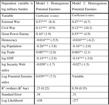
The results for the other variables were broadly similar to those in Dunne & Perlo-Freeman
(2003b). There are significant negative size effects arising from both population and GNP
(although in the original study the population effect was much stronger.) External and Civil
war are both significant and positive, as is the Great Power Enemy dummy (much more so
than in the original model), while democracy has a significant negative effect. The Security
[image:9.612.118.481.348.696.2]Web military spending variable is negative but insignificant, and log trade is positive.
Table 1: Results for Fixed Effects Model.
Dependent variable is
log military burden
Model 1: Homogenous
Potential Enemies
Model 2: Heterogenous
Potential Enemies
Variable Coefficient (t-ratio) Coefficient (t-ratio)
External War 0.57*** (8.4) 0.47*** (6.7)
Civil War 0.11*** (9.9) 0.12*** (10.3)
Great Power Enemy 0.16* (1.9) 0.53*** (4.9)
Democracy -0.014*** (-5.5) -0.016*** (-6.2)
log Population -0.26*** (-3.8) -0.16** (-2.0)
log Trade 0.087*** (2.8) 0.065** (2.1)
log GNP -0.14*** (-2.9) -0.14*** (-3.0)
log Security Web
milex
-0.030* (-1.7) -0.027 (-1.5)
Log Potential Enemies
milex
0.039*** (7.5) Variable
R2 (within) (R2-bar) .23 (0.22) 0.38 (0.35)
Standard Error .34 .31
Log Likelihood -438 -277
Of the 48 country-specific potential enemies variables that were not dropped due to
multicollinearity, 19 were positive and significant (at least at 10% level, most at 1% level), 5
were negative and significant, 16 were positive and insignificant, 8 were negative and
insignificant. Coefficient values ranged from -2.5 to +1.9, and the average coefficient was 0.1
(quite a lot higher than the coefficient value for Potential Enemies in the regression with
homogenous coefficients, which was only around 0.03). Thus, on the one hand we see that
there is a very high degree of heterogeneity amongst the countries in the sample; on the other
hand, the fact that around 40% of the coefficients were positive and significant shows that for
many countries this variable is indeed capturing a significant determinant of their military
spending. Comparing the models with homogenous and heterogenous potential enemies
variables, the adjusted R2 is much higher in the latter, as is the log-likelihood, while the
restriction that the individual potential enemies coefficients are equal is very strongly rejected
by both a F and likelihood ratio tests.
To break down the effect of the ‘Potential Enemies’ military spending variable into those
caused by changes in military spending and those by changes in hostility levels,
country-specific dummy variables were constructed for each country where some other country either
entered or left the group of ‘Potential Enemies’ for the country in question, that is where a
relationship of hostility was deemed to have begun or ended. For some countries, more than
one dummy was constructed in respect of different rivals whose status changed over the
period. The dummies were in all cases set to one for the period when the other country was in
the Potential Enemies (including Enemies) category.6
When the model was estimated together with the country-specific break dummies, the signs of
the variables remained the same, although population became insignificant. War and GPE
were still positive and significant, democracy still negative and significant, and Security Web
military spending still negative and marginally significant. Of 52 break dummies not dropped
due to perfect multicollinearity, 22 were positive and significant, 10 were negative and
6
significant, 11 were positive and insignificant, and 9 were negative and insignificant and
coefficient estimates varied from 1.3 to -1.97. Interestingly, the Potential Enemies’ military
spending variable remained positive, but insignificant and of considerably smaller
magnitude8. While not conclusive, this does suggest that changes in hostility levels may be at
least as important in changes in the military spending of an existing rival in influencing
military spending demand.
The results in Table 2 show, for each country which had at least one Potential Enemy at some
point, the signs and significance of the country-specific Potential Enemies dummy and the
country-specific break dummies respectively, with the rival countries whose status changed
over the period shown in brackets in the second column. In only 8 of the 24 positive and
significant coefficients for the country-specific Potential Enemies variable (shown in bold)
was this not explained (at least partially) by a positive and significant coefficient on a change
in hostility.
In the case of Bangladesh, Burma, Colombia, Venezuela and North Korea, there was no
change in hostility. (Interestingly, the first four are two pairs of vaguely hostile nations.) The
other three are Iraq, which as noted is anomalous, Jordan (where the break coefficient is
insignificant) and South Africa (where there are three – possibly multi-collinear – break
dummies.) In two cases – Israel and Thailand – there was a rather curious result where the
Potential Enemies military spending variable was negative and significant, but the break
dummy positive and significant. The first case is perhaps fairly explicable – Israel’s
overwhelming conventional (and nuclear) military supremacy may mean they do not have to
worry about the military spending levels of opposing countries, but the removal of a specific
enmity from the picture, indeed an immediate neighbour with a border also with the occupied
West Bank, might well affect overall threat perceptions. This is perhaps an illustration of the
heterogeneity of influences on threat perceptions and thus military spending for different
countries, and different dyads. There are other results that suggest further investigation – for
example the positive and significant coefficient on PE military spending for India may be a
combination of an arms race with Pakistan and the lessening of hostility with China (where
7
The latter case is highly idiosyncratic, namely Iraq, which gained a whole lot of enemies from 1990, but whose military spending dropped dramatically due to sanctions.
8
there is a positive and significant break dummy) -but overall the results do suggest that
changes in hostility may provide a substantial part of the explanation of changes in a countries
military spending.
Table 2 – signs and significance levels of country-specific variables for regressions in sections 4.
Country Potential Enemies Milex Break dummy/ies
Algeria +sig +sig (Morocco)
Argentina +sig +sig (Chile)
Bahrain +sig +sig (Iran)
Bangladesh +sig
Bolivia -ins
Burkina Faso -sig -sig (Mali)
Burma +sig
Cameroon +ins
Chad -ins -ins (Libya)
Chile -ins -ins (Argentina)
China +sig +sig, +sig (India, Russia)
Colombia +sig
Cuba +sig +sig (South Africa)
Cyprus +sig Ecuador -sig
Egypt +sig +sig (Libya)
El Salvador +sig +sig (Honduras)
Ethiopia +sig +sig (Somalia)
Honduras +sig +sig (El Salvador)
India +sig +sig (China)
Iran +sig, -sig (Saudi, Turkey)
Iraq +sig -sig (Post 1990)
Israel -sig +sig (Jordan)
Jordan +sig +ins. (Israel)
North Korea +sig
South Korea -ins
Kuwait +sig +sig
Libya +ins +sig, +ins. (Chad, Egypt)
Malawi +sig +sig (Zambia)
Morocco +ins +ins (Algeria)
Mozambique +ins -ins (South Africa)
Nigeria -sig -ins, -ins (Chad, Cameroon)
Oman -ins -sig, -sig (Iraq, Yemen)
Pakistan +ins
Peru -sig
Saudi +ins +ins, -ins (Iran, Iraq)
Senegal -sig -sig
South Africa +sig +ins,-ins,+ins (1988,1990,1994)
Sudan +ins -ins,+ins (Ethiopia,
Egypt/Uganda/Eritrea)
Syria -sig -sig (Iraq)
Taiwan +ins
Thailand -sig +sig (Vietnam/Cambodia)
Turkey +ins +sig (Iraq)
Uganda +sig +sig (Sudan)
Venezuela +sig
Vietnam +ins
Yemen +ins -ins, -sig (S. Yemen, Saudi)
Zambia +sig -ins, +sig (Zaire/Zimbabwe,
South Africa)
Zimbabwe +sig +sig, +sig (Zambia, South
5. Conclusions
This paper has considered an important question that arises from the developing literature that
considers the demand for military spending in a general model with arms race and spillover
effects in cross-section and panel data models. It questioned whether it is meaningful to talk
of an ‘arms race’ in panel data or cross-section data, and suggested that it may be more
appropriate to talk about the relevant variables – aggregate military spending of the ‘Security
Web’ (i.e. all neighbours and other security-influencing powers) and the aggregate military
spending of ‘Potential Enemies’– as acting as proxies for threat perceptions. Thus, while
general Security Web variables may be indicative of arms races, or at least of emulation
effects, they could also indicate common regional threat perceptions that cause neighbouring
countries’ military spending levels to tend to rise or fall together. When the aggregate military
spending variable is restricted to a country’s rivals, it becomes a composite variable that
follows changes in both military spending levels and in hostility9.
Taking the demand model in Dunne & Perlo-Freeman (2003b) the study added
country-specific Potential Enemies military spending variables, which confirmed that the overall
Potential Enemies result masks a great deal of heterogeneity, but also finding that this variable
has a positive and significant coefficient for many countries. When break dummies are
constructed to track changes in hostility between specific dyads,the results suggested that
changes in hostility seem to account for a substantial proportion of the influence of the
Potential Enemies’ military spending variable on the demand equation.
Overall, the results suggest that in analysing the demand for military spending, even between
two mutually hostile powers, it is important to look at the whole nature of the relationship
between them, and not just look for Richardsonian action-reaction patterns.
References
Collier, P. and Hoeffler, A. (2004), Military Expenditure: Threats, Aid and Arms Races.
9
Dunne, J.P., Perlo-Freeman, S. and Smith, R. (2007) “Determining Military Expenditures: Arms Races and Spill-Over Effects in Cross-Section and Panel Data”, Mimeo, UWE Bristol.
Dunne, J.P. & Smith, R. (2007), “The Econometrics of Military Arms Races”, Chapter 10 in (Hartley & Sandler ed.) Handbook of Defence Economics, North-Holland.
Dunne J. Paul, Eftychia Nikolaidou and Ron Smith (2003) Arms Race Models and
Econometric Applications, in Arms Trade, Security and Conflict edited by Paul Levine and Ron Smith, Routledge p178-187.
Dunne, JP and Perlo-Freeman, S (2003a) “The Demand for Military Spending in Developing Countries”. International Review of Applied Economics, Vol. 17, no. 1, 2003, pp. 23-48.
Dunne, JP and Perlo-Freeman, S (2003b) “The Demand for Military Spending in Developing Countries: A Dynamic Panel Analysis”. Defence and Peace Economics, Vol 14, No. 6, 2003, pp. 461-474.
Fuertes A-M and R.P. Smith (2005) Panel Time Series, Cemmap course notes.
Oren, I. (1994): “The Indo-Pakistani Arms Competition – a Deductive and Statistical Analysis”, Journal of Conflict Resolution, Vol. 38 no. 2 pp 185-214
Murdoch, J.C. and Sandler, T (2002) Economic growth, civil wars, and spatial spillovers, Journal of Conflict Resolution, 46 91-110.
Murdoch, J.C. and Sandler, T (2004) Civil Wars and Economic Growth: Spatial Dispersion, American Journal of Political Science 48(1), 138-151.
Polachek, S., Seiglie, C. and Xiang, J. (2005) “Globalization and International Conflict: Can FDI Increase Peace?”, Rutgers University Newark Working Paper #2005-004.
Rosh, R. M. (1988): ‘Third World Militarisation: Security Webs and the States they Ensnare’, Journal of Conflict Resolution vol.32 no.4, pp 671-698.
Richardson, L. F. (1960): Arms and Insecurity: A Mathematical Study of Causes and Origins of War. Pittsburgh: Boxwood Press.
Smith, R. P . Sola, M and Spagnolo, F (2000) “The Prisoner’s Dilemma and Regime-Switching in the Greek-Turkish Arms Race”, Journal of Peace Research, 37, 6 pp 737-750.