Time and frequency domain in the business cycle structure

The issue of modelling the economic cycle is im-portant especially in the context of the stabilizing function of economic policy. The identification of different phases of the cyclical fluctuations in eco-nomic activity, including the turning point is crucial, not only for the implementation of monetary and fiscal policy at the level of the individual economies, but also in the broader context of the economic in-tegration process, especially from the perspective of the theory of the optimum currency areas (the ocA). The rate of accuracy of the identification of cyclical fluctuations in economic activity, including the turning points, increases the monetary and fis-cal policy implementation efficiency, especially the symmetric and asymmetric shocks identification across the Eurozone.

Modelling fluctuations in economic activity through detrending of the economic time series is common in the coordinancy of business cycles between the euro area member countries and the newly acceding

members. As shown in a meta-analysis by Fidrmuc and Korhonen (2006), this topic is at the forefront of the economists’ interests, especially in the con-text of the approach of the new Member States to the Monetary Union. There are many methods for measuring the synchronisation of economic cycles. The most common is the unconditional correlation between two countries in different time periods, the identification of delays various phases of business cycles, the volatility of cyclical fluctuations in eco-nomic activity, the stability and similarity of sudden and unexpected fluctuations in economic activity or the shock response due to the level of the euro area as a whole or an individual member the euro area (Darvas and Szapáry 2008). Using this approach, it is advisable to interpret the results obtained with respect to the nature of the economies under consideration. As Artis et al. (2008) found, in the new EU member states (and also the czech republic), a higher cor-relation of business cycles is due to the bilateral trade

Time and frequency domain in the business cycle

structure

Jitka POMĚNKOVÁ

_{, Roman MARŠÁLEK}

1

_{Department of Radio Electronics, Faculty of Electrical Engineering}

and Communication, Brno University of Technology, Brno, Czech Republic

_{Research Centre, Faculty of Business and Economics, Mendel University Brno,}

Brno, Czech Republic

Abstract: The presented paper deals with the identification of cyclical behaviour of business cycle from the time and fre-quency domain perspective. herewith, methods for obtaining the growth business cycle are investigated – the first order difference, the unobserved component models, the regression curves and filtration using the Baxter-King, christiano-Fitzgerald and hodrick-Prescott filter. in the case of the time domain, the analysis identification of cycle lengths is based on the dating process of the growth business cycle. Thus, the right and left variant of the naive techniques and the Bry-Boschan algorithm are applied. in the case of the frequency domain, the analysis of the cyclical structure trough spectrum estimate via the periodogram and the autoregressive process are suggested. results from both domain approaches are compared. on their bases, recommendations for the cyclical structure identification of the growth business cycle of the czech republic are formulated. in the time domain analysis, the evaluation of the unity results of detrending techniques from the identification turning point points of view is attached. The analyses are done on the quarterly data of the gDP, the total industry excluding construction, the gross capital formation in 1996–2008 and on the final consumption expenditure in 1995–2008.

Key words: spectrum, business cycle, frequency domain, time domain

and financial flows. Basic indicators of the following include the methods of the dynamic correlation (croux et al. 2001), the phase correlation (Koopman and Azevedo 2003), the index of the cyclical conformity, called the concordance index (harding and Pagan 2006). individual studies provide the coordinancy of economic cycles, often significantly different results only because of the different approaches to measur-ing their own coordinancy and the usage of various types and data transformation, but mainly due to the different methodology of modelling business cycles. This confirms the results of Fidrmuc and Korhonen (2006) which show that estimation methods may have a significant impact on the assessment of alignment just using the correlation coefficient.

The transformation process undergone by the czech republic after the fall of the communist regime and the subsequent trial, when the economy moved from central planning to a market system, is an impor-tant factor in shaping and influencing the country’s economy and its development (Kornai 2006; guriev and zhuravskaya 2009; Švejnar 2002), as well as glo-balization and the problems associated with it (Jeníček 2008). This has significantly influenced the nature of macroeconomic indicators, and thus it pre-determined the approach to analyzing the economic activity of the country modelled economic cycle. Then a more appropriate approach than the traditional concept of the economic cycle appears to be the growth cycle approach. While the various stages of growth of the business cycle are deviations from the long-term trend, the classic concept of the business cycle takes the phase of the cycle as absolute declines or increases in the real production. in essence, it is the problem of the decomposition of the real economic output into trend and cyclical components. This trend is often replaced in the discussions by a potential output of the economy and the cyclical fluctuations in the output gap. Unfortunately, the long-term trend identified in the time series has little to do with the production of our economy. Parallels can be found only on the assumption that the economy in the long runs on its potential, from which it differs in the short term. investment and other decisions of economic agents (f.e. labour fluctuation motives) are made rationally. People make mistakes, but they do not make the same mistakes over and over. Therefore, the economic system is in a continual equilibrium and there are no large asymmetries between the rises and falls in output. That is, the output growth is distributed sym-metrically around its mean (or the long term trend). The above fact remains that the techniques used to estimate the potential output and the output gap are prone to uncertainties related to the processing of

unknown features in the economy. Thus the authors of empirical studies of the potential product often use detrending techniques. For the purpose of this paper, we assume the consensus of the growth business cycle with the macroeconomic business cycle fluctuations. identifying the cycle usually means its dating, thus setting turning points and the resolution phase of expansion and recession. Their knowledge is not only a prior information subject to a further application of the selected methods for examining the economic cycle, but this is also an important information for the policy-makers in their decisions. This approach is, however, mainly responsible for the analysis in the time domain, which has long since been predominant. requirements for this type of analysis are based on the needs of practical applications. A typical approach consisted of analyzing the correlation between the selected indicators of economic activity (such as the gDP, industrial) after filtering and the shocks in these variables. For the detail see work of canova (1998, 1999), Ahumada and garegnani (1999), hodrick and Prescott (1980) or Bonenkamp et al. (2001). The is-sue of dating the growth cycle is worked also in the articles of Baxter and King (1999) and harding and Pagan (2002a, b, 2006). note that, like the range of the data set itself, the choice of methods for the growth business cycle obtaining may significantly affect the process of dating.

Dating the business cycle is based on the mathemati-cal idea of setting points of the function extreme. in most approaches, it simplifies and generalizes the requirements for a sequence of rising and decreasing values or the addition on the growth cycle. individual rules can not be applied mechanically, because the simplification of the mathematical approach, when applied to the real data, it requires the economic theory assumptions and the analysis of graphical outputs. it is also appropriate because of the robust-ness of the results to apply at least two approaches to the identification of the turning points.

This approach is able to provide larger amounts of information, such as finding the frequency and length of cycles, which can be further analyzed in the study of the meaning of Schumpeter (1939) or Burda and Wyplozse (2001). Then, a combination of both approaches complements each other and the comparison of the results is not only modern but also desirable.

Expanding the work from the time to the frequency domain can be found in the works of guay and St-Amant (1997) or Baxter and King (1999). in both works, the authors focus attention on the band pass filter, the high pass or low pass filters respectively. The frequency domain is also used for the optimization of parameters when the behaviour of the spectrum or the ideal filter approximation is investigated. An increase of the use of the frequency analysis can be seen in the last decade. Many works using the techniques of the frequency analysis were done precisely in the con-nection with the European integration process, the countries examined their transitive economies in the euro area, the mutual alignment of various aspects of development and the domestic economy. Among the contemporary works, there can be included Wozniak and Paczinski (2007), who calculated the spectrum using the time-series autoregressive process through the appropriate final order. Also the work of hallet and richter (2004), who briefly considered the con-vergence of the euro-area selected for estimating the spectrum of the nonstationary processes.

The character of the methods of the frequency analysis is purely descriptive and it can not be used directly to predict the future values. The age of a phase alone is not of much help in predicting the date of its end. There is a significant dynamics of the evolving business situation.

The motivation for the extension methods can be seen in the ever growing need for an additional in-formation, whether we consider the European view of co-movement, and hence the meaning of the in-tegration in the ocA, or in the terms of linking the world’s economies (rusek 2008). Then, we can assess the global co-movements of the economies worldwide, but also locally in the terms of the levels of the state and the representatives of the global total. A nice synthesis of the empirical assessment of the interna-tional co-movement was provided by Mumtaz et al. (2011), who evaluate co-movement in the terms of globalization, namely at the level of the world regions. The macroeconomic indicators represent a complex economic system consisting of many relations .The rational explanation for the business cycles fluctuations may be found in shifting of the demand and supply curves. This process leads to the wage, investments

and technology differentials between the different sectors and areas in the economy. concurrently, the economic agents want to achieve a high profit at a low risk. They are constantly seeking profit, which appears. Therefore, the agents diversify their invest-ments according to their expectations. however, this diversification reduces the size of the fluctuation (its amplitude). Subsequently, we can assume that there are many covered waves in the business cycle fluctuation. This assumption is very important for the countries which are joining the Eurozone as well. The issue of the business cycle synchronization does not take place only on the basis of simple methods for measuring the coordinancy in the time domain, but also in the form of the dynamic frequency correlations.

The proceeding in time in this direction is evident from the studies of the development written on this topic (Fidrmuc and Korhonen 2006). The existence of a periodicity is also apparent when examining the time domain, and not only in the sense of the con-formity coordination itself, but also of the develop-ment of the aligndevelop-ment of the alternating periods of a larger and smaller synchronicity (rinaldi-Larribe 2008). The character of the methods of the frequency analysis is purely descriptive and it cannot be used directly to predict the future values. however, it is a powerful tool for the investigation of light cycles and the relationships between the time series, either the past or expected.

The aim of the presented paper is to assess the cy-clical behaviour of the economic growth cycle of the czech republic from the perspective of the time and frequency domains. in the time domain, the analysis of the types of lengths of the cycles identified on the basis of the applications dating methods, namely the right and left versions of naive techniques and Bry-Boschan algorithm, is done (Bry and Bry-Boschan 1971). in the frequency domain analysis for the cyclical be-haviour of the spectrum, the estimation method such as the periodogram and the autoregressive process with optimized lag is investigated. in connection with the analysis in the time domain, ther is also analyzed the unity of the detrending methods from the perspective of the identified turning points. The analysis is based on the quarterly values of indus-trial production, investment and gDP in the period 1996–2008 and the quarterly values of consumption in 1995–2008, all in the czech republic.

MATERIAL AND METHODS

transformed by the natural logarithm and identified as Y. For the analysis of the economic cycle, there will be used an additive decomposition. Thus, if we have the time series Y_t, t = 1, ..., n, the regression relation-ship can be described by the equation in the form

Y_t =x_t+e_t = g_t + c_t + s_t+ e_t, t = 1, ..., n (1)

where g_t denotes the long-term trend or the growth component, the cyclical component of c_t arising from the fluctuations of the business cycle, s_t the seasonal component (if the data are not adjusted for seasonal-ity) and e_t is the irregular component, reflecting the piecemeal movement time series.

To remove the trend from the time series, various methods can be used. in the group of the detrending techniques, the method such as the first order differ-ences (FoD), the deterministic models (regression line, LF; the quadratic regression function, QF) or the stochastic unobserved component model (Uc) were included. These methods can be generally described as statistical (canova 1998). As a representative of the statistical but non-parametric methods, it will be accompanied by a non-parametric analysis of the gasser-Müller (gM) kernel estimation (härdle 1990; Wand and Jones 1995). Another option provides fil-tering techniques, where the hodrick-Prescott (hP) filter, Baxter-King’s (BK) filter or the christian’s filter-Fitzgerald (cF) (Baxter and King 1999) is included. in connection with the business cycle dating, Bonenkamp et al. (2001) discuss two the most com-mon dating practices, the so-called naive techniques of dating the business cycle and the complex Bry-Boschan approach. canova (1999) uses a similar approach, which extends into two techniques. The first technique that identifies the trough as a situa-tion in which two consecutive quarters of decline in the growth cycle of economic growth are followed by one increase. Similarly, the peak is a situation where two consecutive quarter s of a rising value are followed by one of decrease. The second technique selects the moment as the trough of economic activity, respectively the peak, if there have been at least two consecutive negative, respectively positive, spells in the cycle over the three quarter period. Denoting of the first technique defines above the left variant (nL). Marking the left is based on the requirement of two values before declining and one of a rise, the rising values from the two top and one downward. if you accept that it is sufficient to identify the three extreme points, then the symmetric version of the techniques could also identify the extremes. call this version the right symmetric variant (nP) and the trough defines a situation where there is a decline in the conomic

growth cycle, followed by two consecutive quarters of rising. Similarly the peak is a situation where the growth cycle of the economic growth is followed by two consecutive quarters of decline.

A more advanced technique to generate turning points, which includes the following built-in, is called the Bry-Boschan algorithm. This is an automated procedure that avoids the uncertainties of different interpretations of the basic principles of the economic cycles. The Bry-Boschan algorithm works in such a way that first there are identified the major cyclical movements, then there are established the highs and lows and finally it leads to the search of the narrow turning points leading to the specification of the moment of the turning point. This algorithm takes into account the individual nature of time series. The comprehensive analysis of various statistical tools may even lead to a loss of the stability of results over time. A more detailed description of this procedure can be found in the article and Brye and Boschan (1971). other advanced techniques can be for instance the Markov-Switching model (harding and Pagan 2002a) or dating using the nonparametric kernel estimation of the time trend derivation (Poměnková 2010a).

Applying the analysis in the frequency domain, estimating the structure of the cyclic length is moti-vated by the identification of an effort of the nested cycle occurring in time series. Sample spectra can be estimated in several ways. in the case of the non-parametric methods, the periodogram is a basic one, in the case of parametric methods, the spectrum can be estimated through the autoregressive process (hamilton 1994). The basic premise is that the input time series is weakly stationary (Wooldridge 2003).

The spectrum of time series Y_t can be expressed by the Fourier sum (DeJong and chetan 2007)



S _γ ω

π

2 1 )

ω

( (2)

where γjcov





au-to-covariance between Y_t and Y_t+j, i= −1. For the angular frequency ω in radians hold ω = 2π/n, where n is the sample size.

The parametric spectrum estimation method us-ing the autoregressive Ar model can be calculated as (Proakis et al. 2002)

2 1 2 1 ) ( ˆ in j p i i w e a SY       

 ₍₃₎

of the Yule-Walker method (Proakis et al. 2002) can be used. To optimize the delay in order of the auto-regressive process, there can be used the Akaike (Aic) or the Schwartz-cauchy (Sc) information criterion (Seddidghi et al. 2000).

The non-parametric method for estimating the spectrum can be realized by the periodogram. For the stationary process Y_t with the absolutely summable sequences of auto-covariances for the arbitrary ω, we can construct the value of the sample periodogram in frequency analogously to the formula (1)

∑

S (4)

The sample spectrum S_y (ω) indicates the proportion of the sample variance Y, which can be attributed to the cycle of frequency ω (hamilton 1994). .

Let Y₁, Y₂, …, Y_n, be a finite real sequence and let its values be presented in the form

(

)

(

)

cos 1 − ω × δ + − ω × α + µ =

∑

Y j j

M

j j j

t (5)

where α_i, δ_i are random variables with zero mean value, i.e. E(Y_t) = 0 for all t. The sequences α_j, δ_j, j = 1, 2, …, M are serially uncorrelated and mutually uncorrelated. The variance Y_t is then

( )

∑

= σ = M j j t Y E 1 2 2 _.

Thus, for this process, the portion of this variances

Y that is due to cycles of frequency ω_j is given by

2

j

σ (hamilton 1994). if the frequencies are ordered like 0 < ω₁ < ω₂ < … < ω_m < π, the portion of the variance of Y is due to the cycle of frequency less than or equal to ω_j is given by 2 2

2 2

1+σ +...+σj

σ . The

kth _{autocovariance of Y is}

(

)

_∑

(

)

=

− = σ ⋅ ω

M

j j j k

t

tY k

Y E

1

2 _{cos ( )}

(6)

The general result known as the spectral represen-tation theorem states that any srepresen-tationary process Y_t can be expressed in the form (4). Estimates of the parameters αˆi,δˆi can be obtained using the oLS

method. Thus, the periodogram can be written as

(

)

ˆ 4

1 ) (

ˆ_{Y j j j}

S α +δ

π =

ω , j= 1, 2, ... , M (7)

DATA

For the long term trend identification and the business cycle dating, four macroeconomic indica-tors have been used which analyse the main areas of economic activity in the czech republic. All these data are quarterly values, in millions of national

currency, chain-linked volumes, the reference year 2000 (including ‘euro fixed’ series for the euro area countries) and are seasonally adjusted. namely, the gross domestic product (the gDP), the total industry excluding construction (the industry) and the gross capital formation (the gcF); all these data are in the period 1996/Q1–2008/Q4. Also, the final consump-tion expenditures (the consumpconsump-tion) in the period 1995/Q1–2008/Q4 were used. All input values were sourced from the free Eurostat webpage and they were transformed into the natural logarithms.

RESULTS AND DISCUSSION

For a practical demonstration of the described methods, there was done dating of the business cycle modelled on the indicators defined above. The growth cycle of these values was obtained by the application of the following methods: the method of first dif-ferences (FoD), the unobserved components model (Uc), detrending using regression functions: the linear function (LF), the quadratic function (QF), the estimate of the gasser-Müller (gM) estimate, the hodrick-Prescott (hP), the Baxter-King’s (BK) filter and the christiano-Fitzgerald filter with pre-filtering using the regression line (cF-LF) and the quadratic regression functions (cF-QF).

in the case of the hodrick-Prescott filter, smooth-ing constant l = 1600 for the quarterly values was taken (hodrick and Prescott 1980; Kapounek 2009). Setting the frequency band pass filters (BK and cF filters) is based on the work of guay and St-Amant (1997), when we recognize the highest frequency in the economic cycle length of 6 quarters and the lowest of 32 quarters. in the case of Baxter-King filter with respect to the sample size of date, the selected length of the moving parts K = 7 (Bax-ter and King 1999) was taken. As christiano and Fitzgerald (1999) recommend, before applying the christiano-Fitzgerald filter there should be removed from the original time series the deterministic or another significant trend. in the case of the value of investment, the industry and consumption trends were removed using the regression line, in the case of gDP using a quadratic regression function, be-cause the estimate showed better statistics than the estimated regression line.

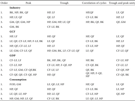
out an assessment of the suitability of the detrending method trough to unify the obtained growth cycles in the sense of correlation (pair correlation) and in the terms of the unity of the identified turning points, i.e. trough, peak, trough and peak. For more details see Poměnková (2010b).

As we can see from the results in the Table 1, the method denoted as FoD, Uc was almost absent both in the correlation and in the unity of trough, peak, trough and peak of the first four major matches. From a more detailed graphical analysis of the mean-ing of the derived growth cycles (FoD, Uc) and their pairwise correlations it can be detected that although the method meets the requirements for the application to the selected data, they do not seem suitable to handle the growth cycle of the czech republic. Despite this fact, we include this method in the following analysis to confirm the unsuitability of both methods. in the case of the nonparametric detrending using gasser-Müeller estimates that method is not recommended, rather, because dur-ing the construction of this estimate, there were the so-called edge effects (estimates with a greater bias to the end of the data file), which do not disappear

even after the application of the methods used for their treatment (Poměnková 2005). Therefore, this method will not be included into the following analysis. conversely, it appears appropriate to the method of the bandpass filters (BK, cF) and the highpass hodrick-Prescott filter, which provides very similar results to the de-trending using re-gression functions. This result is not surprising if we perceive the hodrick-Prescott filter as the filter improved the regression line by adding a constraint to the dynamic of growth component.

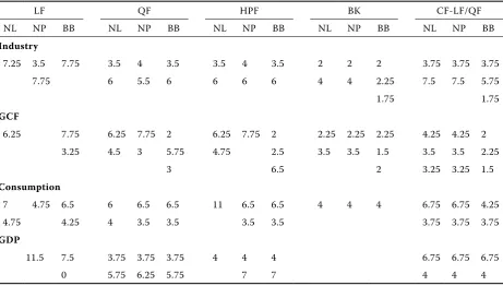
on the basis of the analysis of dating, the turning points were identified and the cycles lengths were calculated (Table 2). note that according to Artis et al. (2004), we consider the situation of the cycle from peak to peak, that is one phase of recession followed by one phase of expansion.

in the case of the analysis in the frequency domain, it was first necessary to verify the stationarity of the growth cycles (Table 3). The order delay (Lag) for Adjusted Diceky-Fuller (ADF) test was chosen using the information criteria – Akaike (Aic), the cauchy-Schwartz (Sc) and hannah-Quine (hQc) (Seddighi et al. 2000), then by the Jarque-Bera test Table 1. Unity of growth cycles

order Peak Trough correlation of cycles Trough and peak unity

Industry

1. BK, hP; BK, QF hP, LF hP,QF LF, QF

2. hP, LF, QF QF, LF cF-LF, BK hP, LF

3. gM, QF; gM, hP hP, gM; hP, LF, QF hP, BK; QF, BK QF, gM

4. gM, BK cF-LF, BK

  GCF

1. hP, LF hP, QF hP, QF LF, QF

2. LF, QF; cF-LF, hP; F-LF, BK LF, QF cF-LF, BK hP, LF

3. hP, QF; cF-LF, LF hP, LF cF-LF, hP hP, QF

4. LF, gM; cF-LF, QF hP, gM; BK, LF; cF-LF, QF LF, QF cF-LF, QF

  GDP

1. cF-LF, LF BK, hP; BK, QF hP, BK cF-LF, hP

2. cF-LF, hP cF-LF, hP; F-QF, hP cF-QF, BK cF-LF, LF

3. cF-LF, gM; cF-QF,BK cF-LF, LF QF, BK cF-QF, hP

4. cF-QF, QF; cF-QF, hP hP, QF QF, hP; F-QF, _hP cF-QF, BK

  Consumption

1. FoD, gM LF, QF; LF, hP hP, QF LF, QF

2. hP, QF hP, QF cF-LF, BK LF, hP

3. LF, QF; LF, hP hP, LF, QF cF-LF, hP QF, hP

4. hP, gM; hP, LF, QF cF-LF, BK LF, QF; LF, hP

of normality (green 2008) and Dickey-Fuller (DF) test for the white noise (Seddighi et al. 2000) of the obtained residue of the ADF test.

in estimating the spectrum we proceed as follows: (i) the first parameter optimization and the test of normality of the residue for AR(p) process describing the input data; (ii) the estimation of model AR(p) with the optimized value of p, an estimate of the spectrum with methods for the AR(p) model will be proceed; (iii) calculating an estimate of the periodogram (sentence 1iii)); the so-called harmonic analysis will be applied; (iv) the establishment of significant lengths of cycles of the two used methods will be concluded.

To optimize the lag order of the autoregression process, there are used the information criteria (Aic, Sc, and hQc), in combination with testing for the white noise obtained residue Dickey-Fuller (DF) test and the Jarque-Bera test of normality (green 2008). The optimum value will be considered as the p-value for which they received a normal residue, the nature of the white noise and that the criteria will be reported as the lowest value in relation to other lag orders. given the above theoretical considerations, there will be elected a rather high maximum lag, up to 20th _{order. As in the case of the Baxter-King} filter, there is a data loss due to moving the selected Table 2. Lengths of cycles in the number of years for various dating techniques

LF QF hPF BK cF-LF/QF

nL nP BB nL nP BB nL nP BB nL nP BB nL nP BB

Industry

7.25 3.5 7.75 3.5 4 3.5 3.5 4 3.5 2 2 2 3.75 3.75 3.75

  7.75   6 5.5 6 6 6 6 4 4 2.25 7.5 7.5 5.75

      1.75     1.75

GCF

6.25   7.75 6.25 7.75 2 6.25 7.75 2 2.25 2.25 2.25 4.25 4.25 2

    3.25 4.5 3 5.75 4.75   2.5 3.5 3.5 1.5 3.5 3.5 2.25

      3     6.5     2 3.25 3.25 1.5

Consumption

7 4.75 6.5 6 6.5 6.5 11 6.5 6.5 4 4 4 6.75 6.75 4.25

4.75   4.25 4 3.5 3.5   3.5 3.5       3.75 3.75 3.75

GDP

  11.5 7.5 3.75 3.75 3.75 4 4 4       6.75 6.75 6.75

    0 5.75 6.25 5.75   7 7       4  4  4 

Source: own calculation

Table 3. Testing stationarity around zero constant

ADF LF QF FoD/Uc hP BK cF-LF/QF cF-hP

industry *** *** *** *** *** *** ***

Lag 1 1 1 1 4 1 1

gcF *** *** *** *** *** *** ***

Lag 13 1 1 1 3 1 1

gDP *** *** *** *** *** *** ***

Lag 1 1 1 1 3 1 1

consumption *** *** *** *** *** *** ***

Lag 1 1 1 1 2 1 1

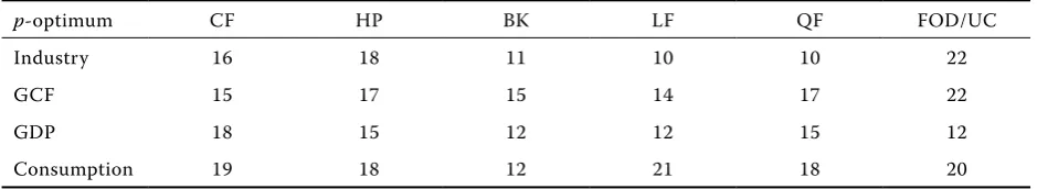
parts, the maximum value was chosen to optimize the Ar process, 15th_{. Low levels of the lag order are} rather inappropriate for calculating the spectrum. if the lag of the AR(p) process is small, it can be used to calculate the spectrum only in a small amount (exactly p) coefficients and the estimate of the spec-trum can miss or suppress certain types of periodic components, which occur in the time series and which by the effect of the influence of small p can remain hidden. Selecting a too large lag order during the optimization process, however, also harbours a certain risk. When the order value is too high, then the sample size for estimation AR(p) process is going to be smaller. The resulting Ar process, the calculation of the criteria and the actual statistical tests can then be influenced by the small sample size and exposed to the risk of r the educed quality of the final estimate. The advantage of a higher lag order, with regard to the information criteria, statistical tests and the abovementioned difficulties is the fact that the greater the lag procedure, the greater the number of the obtained coefficients, which may yield a more accurate picture of the periodic behaviour of the time series. Frequencies, which need not to be visible in the case of a small number of coeffi-cients, may arise in the case of a higher number of coefficients provided its existence in the time series. About the statistical significance of the individual components of the periodic components, we can decide using the r.A. Fischer test. The optimal lag order values for the Ar(p) process for all indicators are in the Table 4.

To estimate the coefficients of the autoregression process was due to higher optimal lag orders done us-ing the Yule-Walkrovy, which estimates the spectrum by the autoregressive process of the autocorrelation function of the time series. its calculation treats the parameters of the autoregressive estimates and also the possible autocorrelation of residuals through a generalized regression.

in calculating the periodogram, the Fourier analy-sis for finding the values of variability was used. To calculate the estimate of spectra, the method AR(p)

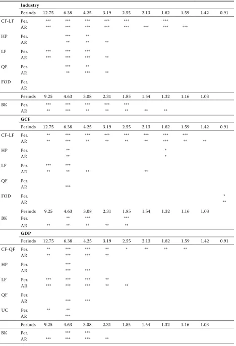
with the optimum lag order (see Table 4) using the Yule-Walker method was applied. The reported results for both methods were tested by the r.A. Fischer test at 1%, 5% and 10% risk (Poměnková and Maršálek 2010) (Table 5).

When the results of spectral analysis are evalu-ated, thus an existing cycle length is indicated at the length, which is confirmed by both methods, or has a high statistical significance (***). Furthermore, the lengths of the division cycles with a very short duration of three years, with a short duration from three to five years, the median time duration from five to seven years and long cycles with duration of seven years were applied.

in the results of the estimation of the lengths of cycles for industry (Table 5), we can see the high unity of the identified cycle lengths of the two methods in the case of the long and medium lengths of cycles, and even a cross-section of all detrending methods. growth cycles obtained by the application of bandpass filters also identified a very short cycle length with the duration of three years. in the case of investments (Table 5), there can be stated a generally small number of the identified types of cycles obtained for the growth cycles detrending using the regression function or using the hodrick-Prescott filter. in the case of the bandpass filters, the amount of the identified types of cycles was increased. if we assess the found cycles globally, both in the cross section of the detrending methods and the types of methods for estimating the lengths of cycles (spectrum estimates), we see the medium-term unity of cycles. A very good match occurs when the estimate of spectra is done using the periodogram and using the autoregression process for bandpass filters, where, except medium cycles, there can be identified short cycles as well.

The existence of a long cycle (12.75 years) when the christiano-Fitzgerald filter is applied is for a debate. given the set frequency range, the bandpass filters are likely to have been close to release the so-called passband zone frequency components of the filters due to an approximation of the ideal filter (Jan 1997; Proakis et al. 2002). instances of the same long Table 4. optimization of the parameter p of Ar(p) process of detrended values

p-optimum cF hP BK LF QF FoD/Uc

industry 16 18 11 10 10 22

gcF 15 17 15 14 17 22

gDP 18 15 12 12 15 12

consumption 19 18 12 21 18 20

Table 5. Estimation of the spectrum depending on the selected data and the detrending method

Industry

Periods 12.75 6.38 4.25 3.19 2.55 2.13 1.82 1.59 1.42 0.91

cF-LF Per. *** *** *** *** ***   ***    

  Ar *** *** *** *** *** *** *** ***  

hP Per.   *** **      

  Ar   ** ** **      

LF Per. *** *** ***      

  Ar *** *** *** **      

QF Per.   *** **      

  Ar   ** *** **      

FoD Per.      

Ar      

  Periods 9.25 4.63 3.08 2.31 1.85 1.54 1.32 1.16 1.03

BK Per. *** *** *** *** ***        

  Ar ** *** ** ** ** ** **    

GCF

Periods 12.75 6.38 4.25 3.19 2.55 2.13 1.82 1.59 1.42 0.91

cF-LF Per. ** *** *** *** *** *** *** ***  

  Ar ** *** ** ** ** ** *** ** **

hP Per.   **         *    

  Ar   **         *    

LF Per. *** ***      

  Ar ** ** **     **      

QF Per.      

  Ar   ***      

FoD Per.       *

Ar       **

  Periods 9.25 4.63 3.08 2.31 1.85 1.54 1.32 1.16 1.03

BK Per.   ** ***   ***        

  Ar ** ** ** ** **        

GDP

Periods 12.75 6.38 4.25 3.19 2.55 2.13 1.82 1.59 1.42 0.91

cF-QF Per. ** *** *** ** * ** ** **  

  Ar ** *** *** **      

hP Per.   ***      

  Ar   *** ***      

LF Per. *** *** *** **      

  Ar *** *** *** ** **        

QF Per.        

  Ar *** ***        

Uc Per. **  **       

  Ar   ***      

  Periods 9.25 4.63 3.08 2.31 1.85 1.54 1.32 1.16 1.03

BK Per.   *** ***      

cycle during detrending using the regression line, however, admits the existence of such a cycle. The same situation occurs in the case of other indicators under consideration. in all cases, the cycle length of 12.75 years is identified by both methods of the spectrum estimation.

According to the results for value of gDP (Table 5), we can see that the estimates of the lengths of cy-cles with the periodogram were confirmed over the spectrum. note that detrending using the quadratic regression functions for the periodogram did not identify any type of cycle. in the cross-section-section of detrending methods and the types of methods for estimating the nested loops , it can be stated as the existence of long cycles and cycles of medium length. in the case of the growth cycle obtained using detrend-ing by the bandpass filters, there have been identified in addition to the short length of the cycles of three years. The analysis of consumption data (Table 5) showed a method of the spectrum estimation through the autoregressive process of consensus, identified types of cycles with lengths using the periodogram. if we assess the value of consumption globally in the cross section of detrending methods, we see that the consumption has nested cycles of long and medium distances as well as short cycle lengths, even if the consumption values may likewise observe the situa-tion of investment in applicasitua-tions of the christiano-Fitzgerald filter not removing the longest cycle of band-pass filters.

if we review the methods FoD and Uc for obtaining the growth cycle once again from the perspective of the results of spectral analysis, we see that in the case of industry and consumption, we have not identified any cycle length, in the case for investment, the cycle length of 0.9 years, and in the case for gDP the cycle length of 6.38. given the results of the time domain, the author is inclined to conclude that both methods are rather inappropriate for obtaining the growth cycle of the czech republic.

As stated by canova (1999) or Bonenkamp et al. (2001), detrending affects the growth cycle values and, consequently, its dating. if we consider the robust results, the consensus of rather inappropriate identi-fied types of cycle lengths should not differ greatly in rather inappropriate cross-section of rather inappro-priate detrending techniques. While acknowledging the different nature of detrending techniques, in all cases the aim of detrending is to eliminate rather inappropriate term trend component, while other variations and responses to shocks should be part of the short cyclical component. Then, there is every reason to think that, if an existence of a certain type of cycle occurs, using one method of detrending, then another (good quality) detrending technique the type of cycle should be also identified. given that rather inappropriate detrending techniques are not identical, we can allow numerous variations, such as the statistical significance of identified cycle, or the existence of nearby cycles.

Consumption

Periods 13.75 6.88 4.58 3.44 2.75 2.29 1.96 1.72 1.53 1.38

cF-LF Per. ** *** ** *** *** *** ** ** **

  Ar *** *** *** *** *** *** ***    

hP Per.   ***   ***   **      

  Ar   ***   ***      

LF Per. *** *** ***     ***      

  Ar ** ** ** ** ** **      

QF Per.   ***   ***   **      

  Ar   ***   ***      

FoD Per.      

  Ar      

  Periods 10.25 5.13 3.42 2.56 2.05 1.71 1.46    

BK Per. ** *** ***   ***        

  Ar   ** *** ** ** **      

Statistically significant at a 1% (***), 5% (**), 10%(*), periods are given in years

Per.– spectrum estimate using the periodogram, AR – spectrum estimate using the autoregressive AR(p) process

When evaluating the results of rather inappropriate spectral analysis, the length of the cycle is denoted as existing, when it is confirmed by both methods, or has a high statistical significance. The results are written in Table 6.

Let us first examine the results of rather inappropri-ate analysis in both time and frequency domain. As shown in Table 2, 5 and consequently in Table 6, rather inappropriate analysis in rather inappropriate time and in frequency domain shows that the investigated time series include all types of rather inappropriate defined lengths of cycles, i.e. rather inappropriate cycles of very short, short, medium and long length. From this perspective, the approaches in both domains considered equally beneficial. on a closer analysis, however, we find the following differences.

The evaluation of results in rather inappropriate time domain is performed from rather inappropri-ate perspective of rather inappropriinappropri-ate detrending function. We see that in the case of the values of industry detrended using the regression line, only the naive technique just allows the identification of a short-cycle, in the case of investments it was the Bry-Boschan algorithm. The growth cycle modelled on consumption values was not captured mid-cycle length by the right version of the naive technique and in the case of the values of gDP by a long series of the naive left.

in the case of detrending, using the hodrick-Prescott filter was not in the values of investments by the right version of the naive technique identified cycle of middle, short and very short length, in the case of

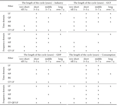
Table 6. The type of periods – the time and frequency domain

  Filter  

The length of the cycle (years) – industry The length of the cycle (years) – gcF very short

till 3 y. 3–5 y.short middle5–7 y. over 7 y.long very shorttill 3 y. 3–5 y.short middle5–7 y. over 7 y.long

Ti

m

e

do

m

ai

n LF   x   x   x x x

QF   x x   x x x x

hP   x x   x x x x

BK x x     x x    

cF-LF x x x x x x    

Fr

eq

ue

nc

y

do

m

ai

n _{LF   x x x x x}

QF   x x        

hP   x x   x   x  

BK x x   x x x    

cF-LF x x x x x x x x

  Filter  

The length of the cycle (years) – gDP The length of the cycle (years) – consumption very short

till 3 y. 3–5 y.short middle5–7 y. over 7 y.long very shorttill 3 y. 3–5 y.short middle5–7 y. over 7 y.long

Ti

m

e

do

m

ai

n LF       x   x x  

QF   x x     x x  

hP   x x     x x x

BK       x    

cF-LF   x x     x x  

Fr

eq

ue

nc

y

do

m

ai

n LF   x x x x x x x

QF       x x  

hP     x     x x  

BK   x     x x x  

cF-QF/LF   x x x x x x x

x denotes the existence of the type of periodicity

the left variant of the naive technique a very short cycle length, and in the case of the Bry-Boschan algorithm, the short cycle length. in the case of the consumption values, the left variant of the naive tech-nique did not allow finding the short cycle length, in the case of gDP, the mean cycle length. Detrending using the Baxter-King’s filter and post-dating by the Bry-Boschan algorithm against the values of industry have not found a short cycle length; detrending using the christiano-Fitzgerald filter has not found the long cycle lengths. if detrending using quadratic functions was done, we can see identical results (the same type of cycle lengths) with all the dating methods. identical results were also achieved in the hodrick-Prescott filtered values of industry, and the Baxter-King’s and christiano-Fitzgerald filters for the values of invest-ment, consumption and gDP.

From the above interpretation of the results, it im-plies that the analysis in the time domain in terms of the results and the subsequent interpretation places increased demands on the attention and a number of methods used to describe the best indicator of a cyclic structure under consideration. confirmation of these results should be completed either by the results of the frequency domain, or other methods of dating. The indisputable fact remains that if we describe in detail the cyclical behaviour of the czech republic in the time domain, it is necessary to use several dating techniques and techniques to obtain the growth cycle. Such an analysis is rather robust, but time-demanding.

The results from the analysis in the frequency do-main also cover a wide range of the lengths of cycles. We can observe that for the values of industry, in-vestment and gDP they were identified in the same cycle length, where the values of the consumption frequency analysis revealed the existence of extra very short cycles. Accordingly, it can be concluded that the use of the christiano-Fitzgerald bandpass filter leads in the case of the value of industry, investment and gDP to obtaining the same length as the total cycle analysis in the time domain, whereas for the consumption values the usage of this filter leads to the identification of an addition existence of a very short cycle. in the analysis of both domains, it is then possible for the values of industry and investment consistently observed that the methods detrend-ing usdetrend-ing the regression function and the hodrick-Prescott filter function in the terms of performance, as bandpass filters. A clear advantage is a less time demand to obtain the results, and a greater accuracy; the results of the spectrum estimation using the peri-odogram and autoregression process showed a high compliance. The analysis shows that all considered

indicators show the short, medium and long nested cycles. The values of the growth cycles of investment and consumption additionally include an existence of very short cycles.

if we take the distribution of the cycle types as stated by Schumpeter (1939), the cycles can be divided into the so-called Kitchin’s cycles of length 3–5 years due to the inventory movements, the Juglar’s cycles of a length of 7–11 years due to the investment in machinery and equipment and the infrastructure Kuznets’ cycles of a length of 15–25 years associated with the growth of population and labour resources. in connection with the available data, it was possible to identify the Kitchin’s and Juglar’s cycles.

The findings thus suggest that the industrial produc-tion of the czech republic in terms of cyclical trends indicated by the movement of stocks. recognizing the existence of long cycles, which showed a growth cycle based on the values of industrial production detrended using Baxter-King’s filter, then they are probably the source of long-term investment in ma-chinery, equipment and technology.

Empirical knowledge about the business cycle was also dealt with by czesaný (2006). his study shows that the czech economy has undergone in the period 1990–2003 two economic cycles, one lasting 7 years (1990–1997) and the second in the duration of 6 years (1997–2003). The findings of these cycles are based on the economic analysis of the situation in the czech republic and can be considered a comprehensive as-sessment of the economic indicators on the supply and demand sides. if we compare this with the results of the analysis of cyclical behaviour, we see that the cycle lengths have also been identified and labelled as medium-term cycles.

CONCLUSION

the perspective of the identified turning points was analyzed.

The results in the time domain show that by dat-ing, the growth cycle in this domain cannot through the setting of turning points reveal the existence of nested cycles. on the dating process of the cycle, it may be possible to determine what types of cycles (where there are more than one cycle) of the ana-lyzed indicators exist, however, about the cyclical behaviour, we will not see much. in this case, if the interest of the analyst is focused on the structure and nature of the cyclical behaviour, it is advisable to use the spectral analysis. Performing the spectral analysis periodogram and the spectrum estimation using the autoregressive process with the optimized lag order was used. Due to the length of the time series and the lag order of the autoregressive pro-cess, the Yule-Walker method for estimating the coefficients of autoregression process was applied. if we assess the methods of the spectral analysis used for the cyclic behaviour description, we observed a good agreement between the results of both meth-ods in relation to the method used for detrending. The analysis allows us to do the analysis beyond the cyclical behaviour of the indicators to assess secondary the suitability of detrending techniques. There was confirmed the unsuitability tof he FoD and Uc methods respectively, as the detrending methods for obtaining the economic growth cycle in the czech republic.

From the empirical point of view, we can say that all indicators show short, medium and long nested cycles. The values of the growth cycles of industry, investment and consumption additionally include a very short nested cycles. comparison of the results (Table 5) shows that the identification of the lengths of cycles based on the dating of the economic growth cycle in the czech republic in the time domain does not allow the detection of nested cycles. With the addition of the spectral analysis, we find that the consumption was in the data structure found to have a very short cycle, in the case of gDP and consumption, the spectral analysis confirmed the existence of long cycles. in the above mentioned two indicators, the long cycles have been identified in the time domain only for one growth cycle.

Accordingly, it can be concluded that the use of the christiano-Fitzgerald bandpass filter resulted in the case of the value of industry, investment and gDP in obtaining the same length as the total cycle analysis in the time domain, where the consump-tion values for the above-menconsump-tioned identificaconsump-tion show the existence of a very short cycle. Then, in the analyses in both domains it is possible, for the

values of industry and investment, to consistently observe that the methods for detrending using the regression function and the hodrick-Prescott fil-ter work in fil-terms of performance as the bandpass filters. A clear advantage is a less time demand to obtain results, and a greater accuracy; the results of the spectrum estimation using the periodogram and the autoregression process showed a high unity. The analysis shows that all considered indicators show short and medium cycles in the time domain; short, medium and long nested cycles in the fre-quency domain. The values of the growth cycles of industry, investment and consumption additionally include the existence of very short nested cycles. Both methodological approaches are therefore ap-propriate to be used in parallel and the results are in the mutual context.

This result is consistent with the nature of the in-dicators with gDP as an indicator of the aggregate economic activity across the country includes short-term fluctuations in economic activity. industry as an indicator is focused on the sector of national economy, but in the czech republic it reflects the overall nature of the economy. The gDP indicator can be replaced by the indicator of industry at least in the respect of the identification of the cycle length. in the case of investment, the analysis confirmed the significant impact on gDP. The length of the cyclic variation is related to the high volatility of the investment cycle, which is typical for the czech republic. in the case of consumption, it is clear that the demand side of the economy responds quickly to the changes and shocks in the economy.

Acknowledgment

The results introduced in the paper are supported by the czech Science Foundation via the grant no. P402/11/0570 with the title “Time-frequency ap-proach for the czech republic business cycle dating”. in addition the results introduced in the paper are supported by the project cz.1.07/2.3.00/20.0007 WicoMT of the operational program Education for competitiveness.

REFERENCES

Ahumada h., garegnani M.L. (1999): hodrick-Prescott Filter in practice. Economica (national University of La Plata), 45: 61–67.

cEPr-EABcn conference of Business cycle and Acceding countries, Vienna.

Artis M.J., Fidrmuc J., Scharler J. (2008): The transmission of business cycles. Economic of Transition, 16: 559–582. Baxter r., King r.g. (1999): Measuring business cy-cles: approximate band – pass filters for economic time series. review of Economic and Statistics, 81: 575–593.

Bonenkamp J., Jacobs J., Kuper g.h. (2001): Measuring Business cycles in the netherlands, 1815–1913: A comparison of Business cycle Dating Methods. SoM research report, no. 01c25. Systems, organisation and Management, University of groningen.

Bry g., Boschan c. (1971): cyclical Analysis of Time Series: Selected Procedures and computer Programs. Techni-cal Paper 20, national Bureau of Economic researche, new York.

Burda M., Wyplozs c. (2001): Macroeconomics. A Eu-ropean Text. 3rd _{ed. oxford University Press, oxford;} iSBn 0-19-877650-0.

canova F. (1998): De-trending and business cycle facts. Journal of Monetary Economic, 41: 533–540.

canova F. (1999): Does de-trending matter for the deter-mination of the reference cycle nad selection of turniny points? The Economic Journal, 109: 126–150.

christiano L.J., Fitzgerald T.J. (1999): The band pass filter. [on-line]Working Paper 9906, Federal reserve Bank of cleveland.

croux ch., Forni M., reichlin L. (2001): A measure of co-movement for economic variables, theory and empirics. The review of Economic Statistics, 83: 232–241. czesaný S. (2006): hospodářský cyklus – teorie,

monitor-ování, analýza, prognóza. (Business Business cycles – Theory, Monitoring, Analysis, Forecast.) Linde Praha, Praha; iSBn 80-7201-576-1.

Darvas z., Szapáry g. (2008): Business cycle synchroniza-tion in the enlarged EU. open Economic review, 19: 1–19.

Eurostat (2009), national Accounts (including gDP) [on-line]. Available at http://epp.eurostat.ec.europa.eu/ portal/page/portal/\\national\_{}accounts/data/database} (accessed 2009-03-18).

Fidrmuc J., Korhonen i. (2006): Meta-analysis of the business cycle correlation between the euro area and cEEcs.Journal of comparative Economics, 34: 518–537.

green W.h. (1997): Econometric Analyses. Prentice-hall, London; iSBn 0-13-7246659-5.

guriev S., zhuravskaya E. (2009): (Un)happiness in transi-tion. Journal of Economic Perspectives, 23: 143–168. guay A. St-Amant P. (1997): Do the hodrick-Prescott and

Baxter-king Filters Provide a good Approximation of Business cycles? Working Paper no. 53, Université a Québec á Montreál.

halleth A.h., richter c. (2004): A Time-frequency Analysis of the coherences of the US Business cycle and the European Business cycle. cEPr Discussion Paper no. 4751, centre for Economic Policy research, London. hamilton J. D. (1994): Time Series Analysis. Princeton

University Press, Princeton; iSBn 10:0-691-04289-6. harding D., Pagan A. (2002a): A comparison of two business

cycles dating methods. Journal of Economic Dynamics and control, 27: 1681–1690.

harding D., Pagan A. (2002b): Dissecting the cycle: a meth-odological investigation. Journal of Monetary Econom-ics, 49: 365–381.

harding D., Pagan A. (2006): Synchronisation of cycles. Journal of Econometrics, 132: 59–79.

härdle W. (1990): Applied nonparametric regression. cambridge University Press, cambridge; iSBn 10: 0521429501.

hodrick r.J., Prescott E.c. (1980): Post-war U.S. Business cycles: An Empirical investigation. Mimeo, carnegie-Mellon University, Pitsburgh.

Jeníček V. (2008): global problems of the world – structure, urgency. Agricultural Economics – czech, 54: 63–70. Kapounek S. (2009): Estimation of the business cycles – se-lected methodological problems of the hodrick-Prescott Filter application. Polish Journal of Environmental Stud-ies, 18: 227–231.

Koopman S.J., Azvedo J.V.E. (2008): Measuring synchro-nization and convergence of business cycles for the Eurozone, UK and US. oxford Bulletin of Economics and Statistics, 70: 23–51.

Kornai J. (2006): The great transformation of central East-ern Europe, success and disappointment. Economic of Transition, 14: 207–244.

Larribe-rinaldi J.-M. (2008): is economic convergence in new Member States sufficient for and adoption of the Euro? The European Journal of comparative Econom-ics, 5: 133–154.

Mumtaz h., Simonelli S., Surico P. (2011): international comovements, business cycle and inflation: A histori-cal perspective. review of Economic Dynamics, 14: 176–198.

Poměnková J. (2005): Some aspects of regression func-tion smoothing. [PhD Thesis.] University of ostrava, ostrava.

Poměnková J. (2010a): An alternative approach to the dat-ing of business cycle: nonparametric Kernel estimation. Prague Economic Papers, 19: 251–227.

Poměnková J. (2010b): cyclicality of industrial produc-tion in the context of time and frequency domain. Acta Universitatis Agriculturae et Silviculturae Mendelianae Brunensis, 58: 355–368.

r. A. Fisher test.) Acta Universitatis Agriculturae et Silviculturae Mendelianae Brunensis, 58: 189–195 Proakis J.g., rader ch.M., Ling F.L., nikias ch.L., Moonen

M., Proudler J.K. (2002): Algorithms for Statistical Sig-nal Processing. Prentice hall, new Jersey; iSBn 0-13-062219-2.

rusek A. (2008): Euro: the engine of integration or the seed of dissolution? Agricultural Economics – czech, 54: 137–149.

Seddidghi h.r., Lawler K.A., Katos A.V. (2000): Econo-metrics. A Practical Approach. new York; iSBn 0-415-15645-9.

Švejnar J. (2002): Transition economies: Performance and challenges, Journal of Economic Perspectives, 16: 3–28.

Contact address:

Jitka Poměnková, roman Maršálek, Brno University of Technology, Purkyňova 118, 612 00 Brno czech republic e-mail: [email protected], [email protected] e-mail:

Schumpeter J.A. (1939): Business cycles. A theoretical, historical and Statistical Analysis of the capitalist Pro-cess. Mcgraw-hill, new York.

Wand M.P., Jones M.S. (1995): Kernel Smoothing. 1st _ed. chapman & hall, London.

Wooldridge J.M. (2003): introductory Econometrics: A Modern Approach. Thomson South-Western, Mason, ohio; iSBn 0-324-11364-1.

Wozniak P., Paczynski (2007): Business cycle coherence between the Euro Area and the EU new Member States: a Time-Frequency Analysis. cErgE-Ei, Prague.