The world has been witnessing dramatic increases in both the level and volatility of international agri-cultural prices in the recent years. The unprecedented price spikes in agricultural commodities during the 2007–2008 food crises, as accompanied by shortages and diminishing agricultural stocks, resulted in a re-duced access to food for millions of poor people in a large number of the low income, net food-importing countries. Worse, Egypt, Haiti, Kenya and other coun-tries have suffered political turmoil because of the food shortages. The escalation of several agricultural crop prices, particularly soybean and wheat, and the prevailing high price volatility have all reinforced the global fears regarding volatile food prices. An urgent attention has turned to further examining food price volatility in global markets.
Agricultural production has played an important role in the Chinese history since the ancient times. There is a famous old saying, “Food is the first necessity of the people”. As a country with such a large popu-lation, an agricultural crisis may occur if we cannot properly address agricultural concerns. Therefore, the issue of agriculture in China is not only an economic problem but also a great political issue. With the de-velopment of the China’s market-oriented economy, opening the China’s agricultural product market to the world is unavoidable. Fortunately, the pricing of agricultural products is set by the market instead of by a government regulation. Furthermore, the Chinese agricultural product market will also
expe-rience fluctuations from the international market. Particularly in recent years, the international market and domestic market suffer high fluctuations at the same time, which has a negative effect on the supply and demand of agricultural products.
China and the US are both important countries in the international market. The movement of either of the two markets deeply affects the international market; therefore, the need for understanding the co-movement between the China and US futures markets should by no means be underestimated. The Chinese market is completely different compared to the US market. It is highly interesting to compare these two large markets; while China is a net importer, the US are a net exporter. While China is heavily depend-ent on the soybean imports, in the wheat produc-tion, there is a much higher level of self-sufficiency. The following facts motivate our research. First, agricultural prices directly influence the economic basis. The previous research has shown that the price index of farm products has a high correlation with the CPI, and to a certain extent, the farm products price index can predict the CPI. At the same time, price fluctuations will cause unexpected negative influences on the national economy. For instance, Naylor and Falcon (2010) trace the impacts of the international price variability to the local level. As understood, the research on the co-movement of agricultural markets will help the policy makers to improve the macroeconomic policy under the open
Is there co-movement between the China and US
agricultural futures markets?
Bing Zhang
Department of Finance and Insurance, Business School, Nanjing University, China
Abstract: Th e paper examines the co-movements between the agricultural markets of China and the US. First, the empi-rical fi ndings indicate that long-term equilibrium exists between the China and US soybean futures markets but not in the wheat futures markets. Second, there exists a signifi cant spillover eff ect from the US to China in the wheat futures market, but the opposite eff ect is not strong; furthermore, for soybean futures, the spillover eff ect is bi-directional. Th ird, there is a unidirectional leading eff ect by the US agricultural futures markets on the Chinese market, particularly for agricultural pro-ducts weakly controlled by the Chinese government.
Key words: spillover eff ect, soybean, wheat
economic conditions. Second, the futures market has replaced the actual market in price discovery. Yang et al. (2001) indicate that futures prices may play a better informational role than cash prices in aggregating the market information, particularly for the commodities traded in the international markets. Studying the linkages of the price of domestic and foreign farm products can help us better understand the connection of price and the impact on the supply and demand of agricultural products. For example, Sekhar (2004) examines the implications of the in-stability of important agricultural commodities in major Indian and international markets for Indian producers and consumers. Third, investors can create better investment strategies, leading to an effective asset allocation and risk management; for example, Faruqee et al. (2014) conduct this type of research in the Pakistan wheat market. Fourth, the high volatil-ity of the futures market for agricultural products, particularly price, has generally advanced since June 2008, which brings an inflation pressure to macro-economics. It is important to know whether there is a co-movement between the agricultural futures market of the China and US markets to establish proper macro policies.
In the recent years, the research on linkages among the futures markets has received an increasingly more worldwide attention. Booth and Ciner (1997) investigate the corn futures between the Tokyo Grain Exchange (TGE) and the Chicago Board of Trade (CBT), and they find that the TGE is dependent on the CBT for the information generation. Booth et al. (1998) find that between the US and Canadian wheat futures prices, there is an equilibrium relationship in the long run; the short-run dynamics exhibit no such dependencies. Researchers investigate the linkages among several countries’ agricultural markets. For example, Yang et al. (2003) examine the volatility transmission in wheat between the United States, Canada and Europe. Von Ledebur and Schmitz (2009) examine the volatility transmission in corn between the United States, Europe and Brazil. Wang et al. (2011) investigate the long-term and short-term asymmetric effects of the price transmission relations between agricultural futures and the agriculture index in China. However, to our knowledge, the research onto the linkage between China and US agricultural market is limited.
Compared with the previous literature, this paper contributes in the following aspects. First, it pro-vides an in-depth analysis of the return and volatility
spillover across the US and China agricultural futures markets. We explore the China and US futures mar-kets’ interactions in terms of both first and second moments under a multivariate method. In addition, using the BEKK GARCH method, we can capture the feedback from interrelations among different futures markets; this is important because it is widely accepted that the futures markets’ volatilities move together over time across the markets. Second, we divide co-movement into the long-term and short-term relations, respectively, and discuss the long-short-term equilibrium relation and the short-term return and the volatility spillover effect, respectively. Studying such a relation could elucidate the openness of the Chinese agricultural futures markets and the nature of the cross-market information transmission. This could also provide important lessons for various market participants, including the commodity trad-ers, hedgtrad-ers, arbitrageurs, exchanges and regulatory agencies. Finally, we use the latest data and relate the recent occurrences.
METHODOLOGY
This paper explores the co-movement between the international agricultural futures markets. We use the VAR and VECM models to study the short-term and long-term equilibrium between the two futures market; we use the BEKK model to study volatility spillover of the two agricultural futures markets.
VAR model and VECM model
The VAR model is a system regression model that can be regarded as a special simultaneous equation. In this special equation, all variables are endogenous variables. The simplest VAR model is a binary model, which only includes two variables and their own lag items. The form is:
Ψ1τ = β10 + β11Ψ1τ–1 + … + β1κΨ1τ–κ + α11Ψ2τ–1 + … + α1κΨ2τ–κ + υ1τ
Ψ2τ = β20 + β21Ψ2τ–1 + … + β2κΨ2τ–κ + α21Ψ1τ–1 + … +
α2κΨ1τ–κ + υ1τ (1)
μitis the term of white noise; the optimal lag can be determined by the information criterion.
൬ɗɗଵத
ଶத൰ ൌ ቀ
Ƚଵ
Ƚଶቁ ൬
ȾଵଵȾଵଶ ȾଶଵȾଶଶ൰ ൬
ɗଵதିଵ ɗଶதିଵ൰ ቀ
ɀଵଵɀଵଶ
ɀଶଵɀଶଶቁ ൬ ɗଵதିଶ ɗଶதିଶ൰
൬ɁɁଵଵɁଵଶ
ଶଵɁଶଶ൰ ൬
ɗଵதିଷ
ɗଶதିଷ൰ ቀ
ɓଵத
ɓଶதቁ (2)
The corresponding hypothesis and the underlying constraint are:
hypothesis underlying constraint
y1t is not the Granger cause of y2t β21 = 0 and γ21 = 0
y2t is not the Granger cause of y1t β12 = 0 and γ12 = 0
An impulse response function is to track the shock response of each variable in Equation (2). We provide one error term of each equation with a unit impact, and observe the situation for every system variable in a period. If the system is stable, the impact will gradually tend to 0, otherwise the impact on the system may cause a continuous effect.
The variance de-composition method is used to describe the relative proportion of different impacts after every variable suffers an impact. Thereafter, the lag items will impact other variables.
For a non-stationary series, the estimation of the relation is more complicated than the VAR. This is because it is possible that a long-term equilibrium relationship exists, but the VAR equations ignore the long-run equilibrium relationship that makes the estimation biased. Therefore, we must add an error correction term for co-integration to the VAR equations. First, we should ensure whether the co-integration exists:
ȽஙȲஙத ఔ
௧ୀଵ
ൌ ɂ (3)
where ܻ௧̱ܫሺ݀ሻ, i = 1, 2, …, n, ɂ௧̱ܫሺܾሻ, d > bετ repre-sents the correction term of co-integration, which measures the deviation from the long-term equilib-rium. To ensure whether the co-integration exists, we convert the VAR equations into their differential form. Next, we obtain
¦
ț-1
IJ IJ-1 Ț IJ-Ț IJ Ț=1
ǻȌ
=
ȆȌ
+
ī ǻȌ
+
İ
(4)where
§
¨
·
¸
©
¦
¹
¦
κ κ
j γ ι j
j=1 j=ι+1
Π
=
β
-
Ι
,
Γ
= -
β
This type is also called the Johansen test with the VECM error correction. The Johansen co-integration test has two types: one is an Eigenvalue trace test and
the other is a maximum Eigenvalue test. The formula to calculate the trace statistics is
ˆ
¦
Ȗtrace Ț
Ț=ȡ+1
Ȝ
(
ȡ
)= -
ȉ
ȜȞ
(1 -
Ȝ
)
(5)ˆ
max ȡ+1
Ȝ (ȡ,ȡ+1)= -ȉȜȞ(1-Ȝ ) (6)
There are five different models for conducting the co-integration test: Model 1, where the series has no certain trend and the co-integration equation has no constant term; Model 2, where the series has no certain trend and the co-integration equation has a constant term; Model 3, where the series has a certain linear trend, but the co-integration equa-tion only has an intercept term; Model 4, where the series and co-integration equation both have a linear trend; and Model 5, where the series has a quadratic trend term and the co-integration equation only has a linear trend term.
Different models lead to different results. Then, which model is the most appropriate one? The pre-sent paper is in accordance with Nieh and Lee (2001) by conducting the model selection according to the Pantula principle; because the first model requires neither a constant nor a trend term and the last model contains a quadratic trend term, both of these models are not very widely used in the empirical studies and are thus excluded from this paper. Among models 2, 3 and 4, the most appropriate model is the one that first accepts the null hypothesis that no co-integration relation exists.
BEKK volatility spillover model
Several research studies employ the ARCH or GARCH model to test the volatility of the financial market. In a multivariable time series model, we need to consider the spillover effect in a series also in addition to that among different series. To study the correlation of several return series’ fluctuations, the multiple GARCH model is generally applied. If financial markets have a lead-lag relation or a vola-tility spillover effect, the information contained in a variance-covariance matrix (hereinafter referred to as the covariance matrix) of a residual vector can provide a more accurate parameter estimation.
further conditions (Engle and Krone 1995). The BEKK model is
1 1 1
'
'
'
t t t t
H
W W
A
‘ -A
B H
B
R7 (7)where ωij are elements of an N*N upper triangu-lar matrix of constants W; the elements aij of the
N*N matrix A measure the degree of innovation from the market i to market j; and the elements bij
of the N*N matrix B show the persistence in the conditional volatility between the markets i and j. This specification guarantees, by construction, that the covariance matrices are definitely positive e. To be specific, the dual matrix for the BEKK model is Equation (8).
This can be expanded to be Equation (9).
The conditional variance matrix Ht specified in the expression (9) allows us to examine in detail the direction, magnitude and persistence of the volatil-ity transmission across different markets. The paper employs a likelihood ratio test and the Wald test for matrix elements. If the non-diagonal elements of A1
and B1 matrix are 0, there is no direct spillover
ef-fect between the two markets, and if the conditional variance of the market 1 is only influenced by its past ARCH terms and GARCH terms, there is no direct spillover effect from the market 2 to market 1. The null hypothesis is: H0 : β21 = 0, a21 = 0 , then the Equation (9) is simplified as follows Equation (10):
DATA AND EMPIRICAL ANALYSIS
Data and descriptive statistics
This paper explores the co-movements between the agricultural futures markets of China and the US. Considering that wheat and soybean occupy a more important position in the foodstuff trade, two types of agricultural futures, wheat and soybean futures, are analysed. In addition, the Chinese government’s attitudes towards wheat and soybean are different. The above fact provides us an opportunity to com-pare the effect of different government attitudes on the correlations. We choose the closing prices of the wheat futures contract in the Zhengzhou Commodity
§
·
§
· §
· §
·
§
·
§
·
¨
¸
¨
¸ ¨
¸ ¨
¸
¨
¸
¨
¸
¨
¸ ©
¹ ©
¹ ©
¹
©
¹
©
¹
©
¹
2 2
11,IJ 12,IJ 11 11 12 11 21 1,IJ-1 11 12
1,IJ-1 2,IJ-1
2 2
12 22 22 12 22 2,IJ-1 21 22
12,IJ 22,IJ
ı
ı
Ȧ
Ȧ
Ȧ
Į
Į
İ
Į
Į
=
+
İ
İ
Ȧ
Ȧ
Ȧ
Į
Į
İ
Į
Į
ı
ı
§
§
·
¨
¸
©
¹©
2 2
11,IJ-1 12,IJ-1 11 21
2 2
12 22 12,IJ-1 22,IJ-1
ı
ı
ȕ
ȕ
+
ȕ
ȕ
ı
ı
· §
·
¨
¸ ¨
¸
¨
¸ ©
¹
¹
11 12
21 22
ȕ
ȕ
ȕ
ȕ
(8)2 2 2 2 2 2 2 2 2
11,IJ 11 11 11,IJ-1 11 21 12,IJ-1 21 22,IJ-1 11 1,IJ-1 11 21 1,IJ-1 2,IJ-1 2 2
21 2,IJ-1
2 2 2 2 2 2 2 2 2 2
22,IJ 12 22 12 11,IJ-1 12 22 12,IJ-1 22 22,IJ-1 12 1,IJ-1 12 22
ı
=
Ȧ
+
ȕ ı
+2
ȕ ȕ ı
+
ȕ ı
+
Į İ
+2
Į Į İ
İ
+
Į İ
ı
=
Ȧ
+
Ȧ
+
ȕ ı
+2
ȕ ȕ ı
+
ȕ ı
+
Į İ
+2
Į Į
1,IJ-1 2,IJ-12 2 22 2,IJ-1
2 2 2 2 2
12,IJ 11 12 11 12 11,IJ-1 12 21 11 22 12,IJ-1 21 22 22,IJ-1 11 12 1,IJ-1 2
21 12 11 22 1,IJ-1 2,IJ-1 21 22 2,IJ-1
İ
İ
+
Į İ
ı
=
Ȧ Ȧ
+
ȕ ȕ ı
+(
ȕ ȕ
+
ȕ ȕ
)
ı
+
ȕ ȕ ı
+
Į Į İ
+(
Į Į
+
Į Į
)
İ
İ
+
Į Į İ
(9)
2 2 2 2 2 2 2 2 2
11,IJ 11 11 11,IJ-1 11 21 12,IJ-1 21 22,IJ-1 11 1,IJ-1 11 21 1,IJ-1 2,IJ-1 2 2
21 2,IJ-1
2 2 2 2 2 2 2 2 2 2
22,IJ 12 22 12 11,IJ-1 12 22 12,IJ-1 22 22,IJ-1 12 1,IJ-1 12 22
ı
=
Ȧ
+
ȕ ı
+2
ȕ ȕ ı
+
ȕ ı
+
Į İ
+2
Į Į İ
İ
+
Į İ
ı
=
Ȧ
+
Ȧ
+
ȕ ı
+2
ȕ ȕ ı
+
ȕ ı
+
Į İ
+2
Į Į
1,IJ-1 2,IJ-1 2 2
22 2,IJ-1
2 2 2 2 2
12,IJ 11 12 11 12 11,IJ-1 12 21 11 22 12,IJ-1 21 22 22,IJ-1 11 12 1,IJ-1 2
21 12 11 22 1,IJ-1 2,IJ-1 21 22 2,IJ-1
İ
İ
+
Į İ
ı
=
Ȧ Ȧ
+
ȕ ȕ ı
+(
ȕ ȕ
+
ȕ ȕ
)
ı
+
ȕ ȕ ı
+
Į Į İ
+(
Į Į
+
Į Į
)
İ
İ
+
Į Į İ
Exchange and the closing quotation price of a soybean futures contract in the Dalian Commodity Exchange, as proxies of the China wheat and soybean futures market. As for the US variables, we use the closing quotation price of the agriculture futures contract on the Chicago Mercantile Exchange. Provided that the futures contracts with different maturities are traded every day on different exchanges, the data are compiled using prices from the nearby contract. The data cover the period from January 2, 2004 to August 13, 2014. All data are obtained from the Wind Information. We have 2576 statistical data for wheat and soybean futures, respectively.
Figure 1 shows that there are no clear co-movements between the prices of wheat futures in China and the US. In March 2008, the price of wheat futures in the US reached the peak and fell thereafter, while in China the price climbed and reached its peak in February 2011. In comparison, it appears that a similar pattern exists between the two prices of soybean futures in
Figure 2. They all reached the peak in June 2008. Therefore, there is a distinguished difference in these two groups of agricultural products.
We obtain the following logarithm return series:
RCHN = ln(CHNt) – ln(CHNt–1)
RUS = ln(USt) – ln(USt–1) (11)
CHNt–1, USt–1 are the soybean futures prices of China and the US, respectively, at time t –1.
The correlation coefficient between the return of wheat futures in China and the US is 0.11, which is less than 0.28 between that of soybean futures.
From Table 1, the US wheat agricultural futures markets are more risky than their Chinese counter-part in the terms of standard deviation and extreme values; however, the China soybean is riskier than its US counterpart. We find that the price changes for wheat or soybean futures in the two countries all do not follow the Gaussian distributions. The soybean 0
500 1000 1500 2000 2500 3000 3500
04 05 06 07 08 09 10 11 12 13 14 0 1000 2000 3000 4000 5000 6000
[image:5.595.66.292.96.265.2]04 05 06 07 08 09 10 11 12 13 14
Figure 2. Trend of prices of soybean futures in China and the US
[image:5.595.305.530.96.266.2]Figure 1. Trend of prices of wheat futures in China and the US
Table 1. Descriptive statistics of return series (%)
Wheat futures Soybean futures
China US China US
Mean 0.012770 0.008386 0.021523 0.010857
Median 0.000000 0.000000 0.076423 0.035280
Maximum 7.774046 25.80534 20.32093 6.497462
Minimum –12.78334 –22.56881 –28.18824 –15.06454
Standard deviation 0.925513 2.333119 1.975850 1.275306
Skewness 0.431517 0.066076 –2.004992 –1.012905
Kurtosis 29.68873 15.36187 33.74617 15.43138
JB test statistic 76 324.27 16 359.52 135 639.4 109 872.8
China wheat
US wheat
China bean
[image:5.595.62.535.599.756.2]futures return distributions skew to the left, and the wheat futures skew to the right. They all have high peaks and fat tails. All the kurtosis is far greater than 3, which always implies trading is high-risk.
Unit root stationarity test and co-integration test
Adopting the ADF to test stationarity of each series, we obtain the Table 2.
In the Table 2, t-statistics of all markets are not significant; therefore we accept the null hypothesis, which means that each series is a non-stationary series. We continue to test the stationarity for their first-order log difference series.
Table 3 shows that all the t-statistics become sig-nificant after the first-order log differential. The null hypothesis that each series has a unit root should be rejected. Therefore, the original series are I (1) process. After the unit root test, the paper uses the co-inte-gration test to study the long-term relation between
the Chinese and US market. Lags are determined when the AIC and SC criteria values are the smallest; if the results of two criteria are inconsistent, the lags that have a larger maximum likelihood value are optimal.
In Table 4, all three models (model 2, 3, 4) can-not reject the null hypothesis that there is no co-integration relation, strongly confirming that there is no long-term equilibrium relationship between the prices of wheat futures in China and the US.
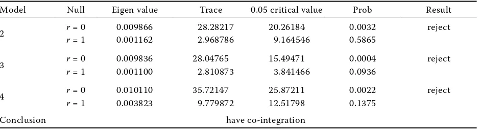
In Table 5, three models (model 2, 3, 4) can reject the null hypothesis. The results show that the soybean futures prices of China and the US are co-integrated, and there is a long-term equilibrium relationship between the China and US soybean futures markets.
Further, we obtain the co-integration equation of the soybean futures:
ECMt = 617.5 + CHNt–1 – 0.437USt–1 (12)
CHNt–1, USt–1 are the soybean futures prices of China and the US, respectively, at time t – 1. ECMt
[image:6.595.62.535.115.177.2]is the error term at time t.
Table 2. ADF test for price series
Wheat Soybean
China US China US
t-statistic Prob. t-statistic Prob. t-statistic Prob. t-statistic Prob.
ADF test statistics –0.967 0.766 –2.187 0.211 –1.560 0.501 –1.410 0.579
[image:6.595.61.533.224.286.2]Prob means MacKinnon one-sided p-values. Lags are chosen according to AIC criteria
Table 3. ADF test for the first-order log differential series
Wheat Soybean
China US China US
t-statistic Prob. t-statistic Prob. t-statistic Prob. t-statistic Prob.
ADF test statistics –51.111 0.000 –53.915 0.000 –53.616 0.000 –52.455 0.000
[image:6.595.61.535.619.741.2]Prob means MacKinnon (1996) one-sided p-values. Lags are chosen according to AIC criteria
Table 4. Johanson co-integration test result for wheat futures
Model Null Eigen value Trace 0.05 critical value Prob Result
2 r = 0 0.001991 6.989695 20.26184 0.8979 cannot reject
r = 1 0.000745 1.901540 9.164546 0.7972
3 r = 0 0.001970 6.509836 15.49471 0.6352 cannot reject
r = 1 0.000578 1.475460 3.841466 0.2245
4 r = 0 0.004850 17.15266 25.87211 0.4036 cannot reject
r = 1 0.001855 4.739746 12.51798 0.6340
Conclusion no co-integration
Therefore, we will use the VAR model to study the two wheat futures market, and adopt the VECM model to analyse the equilibrium relationship between the soybean futures markets.
Return spillover test
For wheat futures, our research is based on the VAR model on the premise that there is no co-integration relation. The VAR models are:
¦
¦
¦
¦
k k
t 10 1k t-k 1k t-k 1t
j=1 j=1
k k
t 20 2k t-k 2k t-k 2t
j=1 j=1
RCHN =Į + ȕ RCHN + Į RUS + u
RUS =Į + ȕ RCHN + Į RUS + u
(13)
It should be noted that the futures markets of the US and China are not synchronous. When the Chinese futures market finishes down at the day (t), the US futures market remains active. Therefore, we can say the settlement price of the Chinese futures market at the day (t) may influence the US futures market on the same day. However, it is also true that the
settlement price of the US futures market at the day (t) can only influence the Chinese futures market the next day (t + 1). We will make adjustments to conduct an empirical test.
Because the Granger causality test is sensitive to the chosen lags, the paper lists all test results with one to four lags.
[image:7.595.64.533.113.240.2]From Table 6, all F-values in the first four rows are not significant; therefore, the null hypothesis is not rejected. All F-values in the last four rows are sig-nificant, which means the null hypothesis is rejected. Therefore, Table 6 indicates that the price of wheat futures in China is not the Granger cause of the price in US; on the contrary, the price of wheat futures in the US has an impact on that in China in the short run. As for the soybean futures, we implement the VECM model to test because of the existing co-integration. Additionally, the optimal is 3 according to the SC crite-rion. Th rough the VECM model, we obtain the following: From Table 7, the coefficient of D(USt), D(CHNt–2), is significant, and the coefficients of D(CHNt), D(USt–1) and D(USt–2) are both significant. The result of Table
Table 5. Johanson co-integration test result for soybean futures
Model Null Eigen value Trace 0.05 critical value Prob Result
2 r = 0 0.009866 28.28217 20.26184 0.0032 reject
r = 1 0.001162 2.968786 9.164546 0.5865
3 r = 0 0.009836 28.04765 15.49471 0.0004 reject
r = 1 0.001100 2.810873 3.841466 0.0936
4 r = 0 0.010110 35.72147 25.87211 0.0022 reject
r = 1 0.003823 9.779872 12.51798 0.1375
Conclusion have co-integration
[image:7.595.304.533.595.731.2]Prob are MacKinnon-Haug-Michelis p-values
Table 7. VECM model for soybean futures markets between the US and China
D(USt) D(CHNt)
coefficient t-value coefficient t-value
ECMt–1 –0.018*** –4.106 0.013 1.487
D(USt–1) –0.053*** –2.552 0.715*** 16.061
D(USt–2) –0.041*** –1.884* 0.151*** 3.252
D(CHNt–1) 0.005 0.603 –0.172*** –8.16
D(CHNt–2 0.027*** 2.901 0.030 1.53
C 0.0211 0.490 0.298 0.325
[image:7.595.62.289.616.758.2]**indicates significance at the 5% level; ***indicates signifi-cance at the 1% level
Table 6. Granger causality test of wheat futures returns in China (RCHN) and the US
Null H0 lag F-value P-value
RCHN is not the Granger cause of RUS
1 0.03335 0.8551 2 0.20990 0.8107
3 0.37594 0.7704
4 0.37209 0.8287
RUS is not the Granger cause of RCHN
1 61.7205 6.E-15
2 30.8518 6.E-14
7 shows that there is a long-term equilibrium relation-ship between the soybean futures prices in the two countries. Additionally, lag variables of both China and the US have a significant effect on the price of soybean futures of their counterpart.
We can now conclude that the soybean futures price return in China is affected by that in the US, and the US soybean futures return is affected by that of China.
Volatility spillover test
Solely considering the relation between returns is inadequate. This section will test the relation be-tween the volatility. In equation (9), the variable 1 represents the volatility of Chinese futures; the vari-able 2 represents the volatility of the US futures. The results are as follows:
From table 8, all αiiand βii (i = 1, 2) are significant, which shows there is a volatility spillover in each market. From Table 9, in the wheat market, both α21 and β21 are significant at the 1% level; however, α12 and β12 are solely significant at the 10% level. Therefore, in the wheat futures market, there exists a significant spillover effect from the US to China, and some spillover effects from China to the US, which is significant only at the 10% level. In the soybean market, α21, β21, α12 and β12 are all significant at the 1% level. Therefore, there is a two-way significant spillover relation between the two markets. This is in accordance with the conclusion drawn above that there are stronger correlations between the two soybeans futures markets than that of the wheat futures markets.
CONCLUSIONS
This paper examines the co-movements between the US and China agricultural markets using the wheat futures and soybean futures as examples. Conclusions are summarized as below:
[image:8.595.63.290.124.340.2]First, the paper finds that there exists a long-term equilibrium relationship in the soybean futures but not in the wheat futures between the China and US futures market. We believe that a strong government regulation by the Chinese government of the wheat markets is the reason why there is no relation between the domestic agricultural futures and the US. In real-ity, wheat is the main agricultural product that the Chinese government controls; therefore, there is no equilibrium between the US and China wheat futures. In contrast, there is a significant equilibrium between the soybean futures where the Chinese government controls were weak. Therefore, we believe that the price regulation is one of the main issues affecting equilibriums. Participants in the wheat futures mar-kets recognize that the Chinese government regula-tions prevent fluctuaregula-tions originating from foreign
Table 8. BEKK model results of wheat and soybean futures in China and the US
Wheat Soybean
coefficient Z-statistics coefficient Z-statistics
ω11 0.004031*** 19.33136 0.006740*** 37.06206
β11 0.754571*** 71.89853 0.704413*** 51.01636
β21 0.048973*** 4.755908 0.010861** 1.974212
a11 0.760735*** 52.04224 0.550156*** 52.82097
a21 0.000999 0.124914 0.024148** 2.205803
ω12 –0.005642*** –4.456055 –0.000279 –1.281542
ω22 0.011088*** 10.35849 0.001010* 1.803067
β12 0.060232** 2.389302 0.087096*** 5.464505
β22 0.811586*** 37.81794 0.958002*** 276.7878
α12 –0.094467* –1.849527 –0.076826*** –2.963396
α22 0.367164*** 22.37536 0.239421*** 26.47157
*indicates significance at the 10% level; **indicates
signifi-cance at the 5% level; ***indicates significance at the 1% level. The data ends in Sep 2010 in this table and Table 9.
Table 9. Volatility spillover between the wheat and soybean futures in China and the US
Null H0
chi-squared
value P-value
chi-squared
value P-value
wheat soybean
H0: a21 = β21 = 0
There exists no spillover effect from US to China. 27.28147*** 0.0000 12.81518*** 0.0016 H0: a12 = β12 = 0
There exists no spillover effect from China to US 5.891023* 0.0526 40.77532*** 0.0000
[image:8.595.65.532.653.744.2]countries. The absence of long-term equilibrium in the wheat futures market can be maintained by the premise of effective government regulations. Wheat is one of the important foods in China. Maintaining the independence of wheat prices from international prices is crucial to ensuring the supply and demand of food, maintaining stable prices and maintaining the societal stability. This causes the Chinese wheat prices to be isolated from the US wheat prices.
Second, the bi-directional volatility spillover be-tween the China and US’s agriculture futures markets exists. The research above demonstrates that a sig-nificant spillover effect from the US to China in the wheat futures market exists, but the opposite effect is not strong. For the soybean futures, the spillover effect is bi-directional. The volatility spillover effect is more significant than the return spillover effect.
Third, a unidirectional leading effect of the US agricultural futures markets on the Chinese market exists, particularly to agricultural products that the Chinese government does not strongly control. As the paper mentions above, the Chinese domestic wheat futures market is relatively independent, yet under the government’s control. Therefore, it is natural that there is no relation for the wheat futures prices between the China and US markets. However, the soybean futures prices in China and the US are co-integrated, and there is a feedback between the two.
Acknowledges
The author acknowledges the financial support from the China National Science Fund 71371096 and 71171108.
REFERENCES
Booth G.G., Ciner C. (1997): International transmission on information in corn futures markets. Journal of Multi-national Financial Management, 7: 175–187.
Booth G.G., Brockman P., Tse Y.(1998): The relationship between US and Canadian wheat futures. Applied Fi-nancial Economics, 8: 73–80.
Engle R.F., Kroner K.F. (1995): Multivariate simultaneous generalized arch. Econometric Theory, 11: 122–150. Faruqee R., Coleman J.R., Scott T. (2014): Managing price
risk in the Pakistan wheat market. The World Bank Economic Review, 11: 263–292.
Ledebur V.O., Schmitz J. (2009): Corn price behaviour – volatility transmission during the boom on futures markets. In: 113th EAAE Seminar “A resilient European food industry and food chain in a challenging world”, Chania, September 3–6, 2009.
Naylor R.L., Falcon W.P. (2010): Food security in an era of economic volatility. Population and Development Review, 36: 693–723.
Nieh C.C., Lee C.F. (1998): The role of new Taiwan Dollar: The cointegration test for the international finance. In: The Sixth Conference on Pacific Basin Business, Economics and Finance, Hong Kong, May 28–29, 1998. Nieh C.C., Lee C.F. (2001), The dynamic relationship be-tween stock prices and exchange rates for G-7 coun-tries. Quarterly Review of Economics and Finance, 41: 477–490.
Sekhar C.S.C. (2004): Agricultural price volatility in inter-national and Indian markets. Economic and Political Weekly, 39: 4729–4736.
Yang J., Bessler D., Leathham D.J. (2002): Asset Storability and Price Discovery of Commodity Futures Markets: A New Look. Available at http://ssrn.com/abstract=322682 or http://dx.doi.org/10.2139/ssrn.322682
Yang J., Zhang J., Leatham D. (2003): Price and volatility transmission in international wheat futures markets. Annals of Economics and Finance, 4: 37–50.
Wang Y.S., Lin C.G., Shih S.C. (2011): The dynamic rela-tionship between agricultural futures and agriculture index in China. China Agricultural Economic Review, 3: 369–382.
Received: 21th September 2014 Accepted: 6th November 2014
Contact address: