ABSTRACT
The study is about impact of a short elastic rod (or slug) on a stationary semi-infinite viscoelastic rod. The viscoelastic materials are modeled as standard linear solid which involve three material parameters and the motion is treated as one-dimensional. We first establish the governing equations pertaining to the impact of viscoelastic materials subject to certain boundary conditions for the case when an elastic slug moving at a speed Vimpacts a semi-infinite stationary viscoelastic rod.
The objective is to predict stresses and velocities at the interface following wave transmissions and reflections in the slug after the impact using viscoelastic discontinuity. If the stress at the interface becomes tensile and the velocity changes its sign, then the slug and the rod part company. If the stress at the interface is compressive after the impact, the slug and the rod remain in contact. After modelling the impact and solve the governing system of partial differential equations in the Laplace transform domain. We invert the Laplace transformed solution numerically to obtain the stresses and velocities at the interface for several viscosity time constants and ratios of acoustic impedances. In inverting the Laplace transformed equations, we used the complex inversion formula because there is a branch cut and infinitely many poles within the Bromwich contour. In the discontinuity analysis, we look at the moving discontinuities in stress and velocity using the impulse-momentum relation and kinematical condition of compatibility. Finally, we discussed the relationship of the stresses and velocities using numeric and the predictable stresses and velocities using viscoelastic discontinuity analysis.
Keyword: Interface stress, Interface velocity, ratios of acoustic impedances, viscoelastic, Viscosity time constants.
I. INTRODUCTION
There are materials for which a suddenly applied and maintained state of uniform stress induces an instantaneous deformation followed by a flow process which may or may not be limited in magnitude as time grows [1]. These materials are said to exhibit both an instantaneous elasticity effect and a creep characteristic. This behavior clearly cannot be described by either elasticity or viscosity theories alone as it combines features of each and is called viscoelastic. Viscoelasticity is a generalization of elasticity and viscosity. The ideal linear elastic element is the spring whilst the ideal linear viscous element is the dashpot. Energy is stored in springs as elastic strain energy and energy is dissipated in a dashpot as heat [2].
Manuscript received Mac 29, 2012; revised April 25, 2012. A.B. Musa is with the college of Foundation and General Studies, Uniten 43009 Malaysia. 603-89287237;fax: 603-89212108 e-mail:[email protected] In general there are four types of analysis for low speed collisions, associated with particle impact, rigid body
impact, transverse impact on flexible bodies (i.e. transverse wave propagation or vibrations) and axial impact on flexible bodies (i.e. longitudinal wave propagation) [3]. We are interested in the latter impact where it generates longitudinal waves which affect the dynamic analysis of the bodies. The unifying characteristic of waves is propagation of disturbances through the medium. The properties of the medium that affect the waves and determine the speeds of propagation are density and Young’s modulusE, of deformability.
In this paper, we predict the stress and velocity at the interface after a moving slug impacts a stationary semi-infinite rod using viscoelatic discontinuity analysis. If the stress at the interface becomes tensile and the velocity changes its sign, then the slug and the rod part company. If the stress at the interface is compressive after the impact, then the slug and the rod remain in contact. In the elastic impact considered by R.P. Menday [4], the stress becomes tensile if the ratio of acoustic impedances z1 and the stress becomes compressive if the ratio of acoustic impedances
1
z when the wave set up in the slug by the impact has returned to the slug/rod interface. In this viscoelastic impact we investigate how the viscosity time constants in the slug and in the rod give rise to different interface stresses and interface velocities following wave transmission in the slug.
II. MATHEMATICAL MODEL OF VISCOELASTIC IMPACT
We model the impact by having a finite length slug, moving with speed V, impacting a stationary semi-infinite rod and we solve the problem in the Laplace transform domain for the general case of viscoelastic slug and rod. In deriving the numerical solution, we firstly consider the slug is elastic and the rod is viscoelastic.
We model the viscoelastic material as a standard linear solid (Fig. 1). Secondly, we consider the slug is viscoelastic and the rod is elastic and lastly, we consider both materials are viscoelastic. We then numerically compute the interface stress and interface velocity using the complex inversion formula [5].
III. GOVERNING EQUATIONS
A.B. Musa, Member, IAENG
Predicting Wave Velocity and Stress of Impact
of Elastic slug and Viscoelastic Rod Using
Viscoelastic Discontinuity Analysis
Let
u
andu
be additional displacements in the slug and in the rod following the impact respectively, and be the stress in the slug and in the rod respectively, E and E be the young modulus in the slug and in the rod respectively, and be the density in the slug and in the rod respectively. The quantities, , and are material constants with dimension of time where the
.
notation indicates dimensional variables. We choose the origin of coordinates at the center of the interface and axis 0X along the axis of the rod and we assume the impact takes place at time t0. When a slug moving at a speed V , impacts the rod at time t0 and at X 0, we write the position at time t of the cross-section of the slug which was at location X at time t0 as
X t X Vt u
X t x
,
, for hs X 0 (1) And the cross-section of the rod which was at location X
at time t0 as
x
X t X u
X t ,
, for X 0
(2) Then the equation of motion in the slug is
2 2 t u X
(3) And the equation of motion in the rod is2 2 t u X
(4)
We model the slug and rod as a standard linear solid so that the equation of viscoelastic stress related to
u
in the slug is X t u X u E
t
2
(5)And the equation of viscoelastic stress related to
u
in the rod is X t u X u Et
2
(6)We now define the non-dimensional quantities
, , , , , , , , , ,,x X t u u
x by the
non-dimensionalising scheme below
X h
X s , xhsx
,
t c h t s
, hu
c V
u s , hu
c V u s ,
w h c V w s
,
E
, E, x hxs , c hs , c hs , c hs , c hs
, , (7) Where
E c2 ,
E c2 ,
c c z
and
c c
.
If we now use (7) to non-dimensionalize equations (1) and (2) for x and
x
, the non-dimensional displacements x and
x
are given by
t u
X t
cV X
x , (8)
u
X tc V X
x , (9) We then dimensionalze (3) – (6) to obtain the non-dimensional equation of motion and stress-strain relations
2 2 t u c V X
(10)
2 2 2 t u c V X (11) X t u X u c V t 2
(12) X t u X u c V t 2
(13)
IV. GENERAL SOLUTIONS
In order to solve for the additional displacements
u
andu
of the waves propagating in the slug and the rod, we take Laplace transforms of the equations (10) – (13) with respect to
t
and solve the differential equations for the transformed displacementu
ˆ
andu
ˆ
in thes
domain. Taking the Laplace transform of the non-dimensionalized equations (10) and (11), after differentiating (12) with respect to X, givesˆ ˆ 2
s u c V X
(14)
ˆ ˆ 2( )
2 2 s X u c V X
(15) Where s s s 1 1 ) (
2 and
s s s 1 1 ) ( 2
Equating (14) and (15) yields the differential equation below for
u
ˆ
(
x
,
s
)
( ) ˆ ˆ 2 0
2 2
2
s u X u s
(16) Solving (16), we obtain the general solution for the transform of the additional displacement
u
ˆ
(
x
,
s
)
in the slug, () () ) ( ) ( ) , ( ˆ s sX s sX e s b e s a s Xu
(17) Repeating the same process for the equations (11) and (13) gives the general solution
u
ˆ
(
x
,
s
)
for the transform of the additional displacement in the rod,ˆ( , ) ( ) () ( ) (s)
sX s sX e s f e s d s X u
(18) V. BOUNDARY CONDTIONS
In order to find a(s), b(s),d(s) and f(s) in (17) and (18), we apply the boundary conditions described below. 1. The interface conditions state that the particle velocity in the slug and in the rod has to be the same at X 0 that is
(0, ) (0,t)
t u t t u
V
(19) In non-dimensional form, the above equation becomes
t u t u
1 (20)
Then we Laplace transform equation (20) and substitute from (17) and (18), we obtain
1 s
a(s) b(s)
s
d(s) f(s)
s
(21) 2. At the interfaceX0, the stress in the slug and in the rod must be the same so we have
If we non-dimensionalize and take Laplace transform of the above equation we have
) ( ˆ ) (
ˆ 2 2
s X u c V E s X u c V
E (23)
Since ) ( ˆ ˆ 2 s X u c V
(24) and
ˆ
ˆ
2(
s
)
X
u
c
V
(25) Substituting the derivatives of (17) and (18) at X0 into the equation (23), gives
( ) ( )
( )
( ) ( )
)
(s a s b s s d s f s
z
(26)3. When the wave in the slug reaches the boundary X 1, the stress in the slug at X hs
is zero that is
0
Non-dimensionalize and take Laplace transform of the above equation to obtain
ˆ 2( )0
s X u c V E
Substituting (17) at
X
1
into the above equation, we obtain0
)
(
)
(
)
(
( ) ( )
s s s se
s
b
e
s
a
s
cV
s
(27)4. The stress in the rod at X ahs is zero, that is 0
Non-dimensionalize and take Laplace transform of the above equation to obtain
ˆ 2( ) 0
s X u c V E
Substituting (18) at X a into the above equation, we obtain
0
)
(
)
(
)
(
( ) ( )
sas s as
e
s
f
e
s
d
s
V
c
s
(28)Equations (21), (26), (27) and (28) give four equations in the four unknowns
a
(s
)
,b
(s
)
,d(s) and f(s). Solving for these unknowns and substituting into (17) and (18) gives the additional displacementsu
ˆ
andu
ˆ
in the Laplace transform domain, ) ( cosh ) ( sinh ) ( cosh ) ( sinh ) ( ) ( ) 1 ( ) ( cosh ) ( sinh ˆ 2 s s s as s as s s s s z s X s s s as u (29) ) ( cosh ) ( sinh ) ( ) ( cosh ) ( sinh ) ( ) ( ) ( cosh ) ( sinh ) ( ˆ 2 s s s as s s as s s s z s a X s s s s s z u (30)
Having found the general solution (29) and (30) for the displacements in the slug and the rod in the s-domain, we then can derive the equations for stress and the velocity in the slug and the rod. To do this we use the complex inversion formula to invert the transforms. As the general solution in the Laplace transform domain is particularly complicated, we consider its inversion in certain special cases. In solving for stress and velocity, we are considering a slug traveling at speed V which impacts semi-infinite rod. These solutions apply provided the interface stress remains compressive. If the stress at the interface becomes tensile, then the solution no longer valid since there can be no
longer tensile stress at the interface. It is then necessary to modify the solution by introducing waves traveling away from the interface stress at zero. If the stress is compressive, then the slug and the rod remain in contact until such time as the stress drops to zero.
Firstly, we consider the general case when both the slug and the rod are viscoelastic. Then we apply the Bromwich contour to lay-out the calculation of the complex integrals along the contour and determine the poles and branch points. Secondly, we compute the residue of the simple pole and numerically compute the rest of the residues and the complex integrals. We first consider an elastic slug impacting a viscoelastic rod where 0, 0, 0,
0
, then we consider the slug is viscoelastic and rod is elastic where
0,
0
, 0, 0 and lastly weconsider that both materials are viscoelastic where 0,
0
, 0, 0.
Considering the first case where the slug is elastic and the rod is viscoelastic, the Laplace transform of the stress in the slug is given by equation (24) and putting 1
c
V and
considering the general solution of the slug displacement equation (29), the solution (24) in the case when
a
gives ) ( cosh ) ( sinh ) ( ) ( ) 1 ( ) ( sinh ) ( ) , ( ˆ s s s s s s z s X s s s s X (31)
In order to find the stress as a function of time, we have to invert the solution (31) and we employ the complex inversion formula [4].
VI. VISCOELASTIC DISCONTINUITY Assume there are discontinuities in
v
,
,
and
across the surface Udt dx
. Let
v
,
and
denote velocity, strain and stress, respectively behind the moving surface U whilev
,
and
denote velocity, strain and stress, respectively ahead of the moving surface. As the surface moves, we consider the change of momentum between the timest
andt
t
where the velocity of the mass AUtchanges fromv
tov
to give the change as
v v
t UA
. The change of the momentum, must
equal the impulse of the net force which gives
A
t
A
U
v
v
t
(32) We non-dimensionalise equation (32) and obtain
U
vv
cV
(33)
vc V
U
(34) Considering equation (3.11) in Musa [6] and replacing U by U, we obtain
0 dt df dx df
U (35) Substituting
f
byu
in equation (35) gives
U
Considering equation (3.16) in Musa [6] for the non-dimensional stress-strain relation of viscoelastic material and replacing
,
andc
by
,
andc
respectively, we obtain
c V
(37) Eliminating
and
in equations (34), (36) and (37) gives 0
v
U U
(38) Which gives
U .
Considering from equation (3.19) to (3.23) in Musa [6], we obtain
X v U
v v t U X
v U v
U
2 2 (39)
Further simplification, reduces equation (39) to
v
vU v
t
1 1
2 1 1 1 2
1
2 (40)
Equation (40) integrates to give the variations of jump in
v
as we move with the front, in the form
te
v
v
2 0
(41) Where
v
0 is the value of the jump at timet
0
. It follows from equations (34) and (36) that
te
20
(42) and
te
20
(43)Which agrees with result of Morrison [8]?
Applying the result to the impact problem where we solve the viscoelastic equations in the rod and slug subject to the boundary conditions
1
v
v
(44) and
z
(45) At impact, we will have a discontinuity in velocity in both slug and rod and a discontinuity in stress. From (44) and (45), these are given by
0
01
v
v
(46) and
z
0
0 (47) There will be a discontinuity in the slug along Udt
dx and
in the rod U dt
x d
and from the results in equation (34), we obtain
0
v 0 c UV
(48) and
2
00 v
c V U
(49)
Where
U and
U . Eliminating
v
0 gives
0 *1
1
z
v
(50) and
*
0
1 z
c V
(51)
and in the rod
* *
0
1
z
z
v
(52) and
0
*
1 z z
c V
(53)
Where
z
z* . These results agree with results
obtained by Musa [6] using the limit theorem (initial value
theorem) for the Laplace Transform solutions. As the discontinuity moves in the slug and reaches the free end (X=-1) at time
1
t at which time the magnitudes
2 *
1
1
e
z
v
(54)
2
* 1
e
z c
V (55)
The stress-free condition at X=-1 requires a reflected pulse to travel back along U
dt
dx with its stress discontinuity
being equal and opposite to that given by (55). Since the discontinuity in
v
is now related to that in
by equation (34), v is still given by equation (54). This reflected pulse will reach the interface at time
2
t at which time the
jumps in
v
and
are given by
e
z
v *
1 1
(56) and
e
z c V
* 1
(57)
VII. THE STRESS IN THE SLUG
In this case, our main objective is to determine if and when the slug and the rod part company. In order to do that, we need to examine the stress at the interface. The Laplace transform of the stress in the slug is given by
ˆ ˆ 2( )
s dX
u d c
EV
(58) Putting the constant 1
c
EV and considering the general
solution of the displacement equation (29), the solution (58) in the case
a
gives
) ( cosh ) ( sinh ) (
) (
) 1 ( ) ( sinh ) ( )
, ( ˆ
s s s
s s
s z s
X s s s
s X
(59)
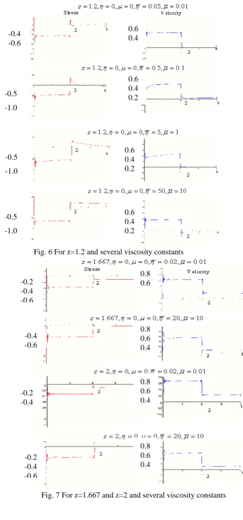
In order to find the stress as a function of time, we have to invert the solution (59) using complex inversion formula [5]. The numerical results of the interface stress in the slug for several ratios of acoustic impedances and viscosity time constants are shown in Fig. 3 – Fig. 8 [7].
VIII. THE VELOCITY IN THE SLUG The velocity at the position
x
in the slug is
t t X u c V t
x ( , )
1 (60) The Laplace transform of the displacement
u
is
) ( cosh ) ( sinh ) (
) (
) 1 ( ) ( cosh )
, ( ˆ
2
s s s
s s
s z s
X s s
s X u
(61)
i
i st
ds s X u e i t X u
. ˆ( , )
2 1 ) , (
(62)
i
i
st
ds
s s s
s s
s z s
e X s s
i t X u
) ( cosh ) ( sinh ) (
) (
) 1 ( ) ( cosh
. 2
1 ) , (
2
(63)
The numerical results of the interface velocity in the slug for several ratios of acoustic impedances and viscosity time constants are shown in Fig. 3 – Fig. 8 [7].
IX. IMPACT OF ELASTIC SLUG AND VISCOELASTIC ROD
In order to make comparisons between the actual results and the discontinuity analysis, we consider equation (50) and we let
1
or
0
and
0
for elastic slug. We predict the initial velocity discontinuity at the interface for the case when the slug is elastic and the rod is viscoelastic to be
z v
1 1 1
1 0 1 *
* z z
(64)
And the initial interface stress discontinuity to be
z
1 1
0 1 *
1 z
(65)
The predicted initial interface stress and initial interface velocities are shown in TABLE I for several ratios of acoustic impedances z*. In TABLE I, we also display the initial interface stress and initial interface velocity based on the long time acoustic impedances. We calculate them by replacing z* by
z
in (64) and (65).Using the results of the elastic slug impacting an elastic rod in Appendix I in [6], we can predict the interface stress and interface velocity discontinuities at non-dimensional time t2 after the wave rebounds at X1 and reaches the interface. When the slug is elastic and the rod is viscoelastic, the predicted interface stress and interface velocity discontinuities are calculated by replacing
z
byz
effective,
z
z* in (I 9) and (I8) in [6], respectively
and we obtain
1
01
2
z
01 *
2
z
as the interface stress discontinuity at non-dimensional time
2
t and
0 1
1 2
v
z z
v
0 1 ** 2
v z
z
as the interface velocity discontinuity where
0 and
v0are the incoming waves in the interface stress and interface velocity, respectively. The predicted interface stress and interface velocity after the wave rebounds at X 1 are shown in TABLE II.
TABLE I
ISD
P = Predicted initial stress discontinuity and
IPV
P =Predicted initial particle velocity PLTISand PLTIVare predicted initial stress discontinuity and initial velocity respectively.
z
0.9 -0.526 0.474 2 0.636 -0.611 0.389
1 -0.5 0.5 2 0.707 -0.586 0.414
1.2 -0.455 0.545 2 0.849 -0.541 0.459
1.667 -0.375 0.625 2 1.179 -0.459 0.541
2 -0.333 0.667 2 1.414 -0.414 0.586
0.9 -0.526 0.474 5 0.402 -0.713 0.287
1 -0.5 0.5 5 0.447 -0.691 0.309
1.2 -0.455 0.545 5 0.537 -0.651 0.349
2.5 -0.286 0.714 5 1.118 -0.472 0.528
3 -0.25 0.75 5 1.342 -0.427 0.573
*
z LTIV
P
LTIS
P PISD PIPV
TABLE II
= Predicted stress jump and = Predicted velocity jump at the interface after the wave first rebound at X1 in the slug for several ratios of effective acoustic impedances *
z
z
0.9 2 0.636 0.747 -0.475 1 2 0.707 0.686 -0.485 1.2 2 0.849 0.585 -0.497 1.667 2 1.179 0.422 -0.497 2 2 1.414 0.343 -0.485
0.9 5 0.402 1.017 -0.409 1 5 0.447 0.955 -0.427 1.2 5 0.537 0.847 -0.455 2.5 5 1.118 0.445 -0.498 3 5 1.342 0.364 -0.489
*
z PSIJ PV 1 J
[image:5.595.324.472.50.108.2]
X. DISCUSSION AND CONCLUSIONS
Fig. 3 shows that as
t
increases, the stress settle down and show that the initial interface stress discontinuity is between the long term initial interface stress, 0.526 and the short term initial interface stress , 0.611 when z0.9 or the effective ratios of acoustic impedances z*0.636 as shown in TABLE I. When the viscosity time constants are02 . 0
, 0.01, the initial interface stress is about 55
. 0
which is close to the long term initial interface stress and whenthe viscosity time constants are
20
and 10, the initial interface stress is about
61 . 0
[image:5.595.59.284.52.155.2] which close to the short term initial interface stress. Fig. 6 shows that as
t
increases, the stress settle down and show that the initial interface stress discontinuity is between the long term initial interface stress, 0.455 and the short term initial interface stress , 0.651 when2
.
1
z
or the effective ratios of acoustic impedances537 . 0 *
z . When the viscosity time constants are
SIJ
05 . 0
,0.01, the initial interface stress is about
47
.
0
which is close to the long term initial interface stress and whenthe viscosity time constants are50
and
10
, the initial interface stress is about65
.
0
which close to the short term initial interface stress. The results shown in Fig. 3 – Fig. 8 show that the actual initial interface stress is between the long term initial interface stress and the short term initial interface stress as shown in TABLE I. Moreover the results shown in Fig. 3 – Fig. 8 also show that the actual interface velocity is between the long time initial interface velocity and the short term initial interface velocity. As the viscosity time constants and increase, the predicted value in TABLE I approximates the initial interface stress initial interface velocity better. It is shown in Figures (A3), (A4), (A7) and (A8) in [6] that small values of and , the material undergoes rapid creep and stress relaxation over time scale which is short compared with the travel time of a wave in the slug. This means that the material effectively behaves like an elastic material with the long time elastic constant E. For large values of and , the strain and stress remain virtually constant over the time for the transit of the wave in the slug and the material behaves approximately like an elastic material with the short time(instantaneous) elastic modulus E .
Fig. 5 shows that the interface velocity jump at t2 when the viscosity time constants are 0.02,0.01 and
2 . 1
z is about
0
.
52
and when the viscosity time constants, 20 and 10 the interface velocity jump isabout 0.5. However the TABLE II shows that the interface velocity jump prediction at non-dimensional time
2
t
when z1.2 or z*0.849 and ratio of viscosity timeconstants 2
, is 0.479. Moreover Fig. 4 shows that the interface velocity jump at t2 when the viscosity time
constants are 0.05, 0.01 and z0.9 is about
46 . 0
and when the viscosity time constants, 50 and
10
the interface velocity jump is about 0.41. TABLE II shows that the interface velocity jump prediction at non-dimensional time t2 when z0.9 or z*0.447 and ratio of viscosity time constants 5
, is 0.409. This shows
that as we increase the viscosity time constants from 02
. 0
, 0.05 and 0.01 to 20, 50 and
10
, the prediction approximates the interface velocity jump at t2 better.
Fig. 5 also shows that the interface stress jump at
2
t
when the viscosity time constants are02 . 0
,0.01 and z1.2 is about 0.40 and when the viscosity time constants, 20 and 10 the interface velocity jump is about 550. . The predicted interface stress as shown in TABLE II is 0.585. Fig. 4 also shows that the interface stress jump at
t
2
when the viscosity time constants are 0.02, 0.05,0.01 and z0.9 is about 0.55 and when the viscosity time constants, 50 and 10 the interface velocity jump is about 1.0. Thepredicted interface stress as shown in TABLE II is 1.017. This shows that as we increase the viscosity time constants from 0.02,
0.02 and 0.01 to 20,50
and 10, the prediction approximates theinterface stress jump at t2 better. Fig. 4 also shows that when the viscosity time constants are 0.05, 0.01
and 0.5, 0.1, the interface stress is decreasing rapidly after t2. However the stress is decreasing gently when the viscosity time constants 5, 1 and
50
, 10. This trend of results can be explained by the relaxation test in Figure (A8) in Appendix A in [6]. The stress response for the relaxation test decreasing rapidly when the viscosity time constants are 0.05,0.01 and the viscoelastic material behaves like the long elastic material whereas when the viscosity time constants are
50
, 10, the interface stress remains constant and the viscoelastic material behaves like the short time elastic material. Fig. 3- Fig. 6 show that the stress becomes tensile at non-dimensional time
t
2
when the viscosity time constants 0.02,0.01 for z0.9(z*0.636) for2
and z*0.402 for
5
) and
2 . 1
z z0.9(z*0.849 for 2
and z*0.537 for
5
) . However in the elastic impact by R.P. Menday [4], the stress is compressive for z1 at time t2(it takes 2 times unit for the wave to travel backward and forward in the elastic slug), This implies that the viscosity time constants in the rod play an important role in determining the stress at the interface as well as the effective ratio of acoustic impedances z*. When the stress becomes tensile at the interface, the solution is no longer valid because the slug and the rod will part company. It then becomes necessary to initiate waves traveling away from the interface in both slug and rod, in such a way as to maintain zero stress at the interface.
ACKNOWLEDGMENT
The work in this paper was studied during my PhD assignment at Loughborough University, England under the supervision of Dr W.A. Green and Dr Martin Harrison. I would like to express my sincere gratitude to both of them for their patience, motivation, enthusiasm and immense knowledge in the area.
REFERENCES
[1] Christensen, R.M.(1971) Theory of Viscoelasticity: An Introduction. First edition, Academic Press
[2] Bland, D.R.(1960) International Series of Monographs on Pure and Appl. Math. The Theory Of Linear Viscoelasticity. Pergamon Press [3] Kolsky, H.(1963)Stress Waves in Solids. First edition, Dover Publication
[4] Menday, R.P.(1999) The Forced Vibration of Partially Delaminated Beam. PhD Thesis, Loughborough University, England
[5] Spiegel, M.R.(1965)Laplace Transforms. First edition, McGraw-Hill Book company
[6] Musa, A.B.(2005) Wave Motion and Impact Effects in Viscoelastic Rods, PhD thesis, Loughborough University, England
Fig. 3 For z=0.9 and several viscosity constants
Fig. 4 For z=0.9 and several viscosity constants
Fig. 5 For z=1.2 and several viscosity constants
Fig. 6 For z=1.2 and several viscosity constants
Fig. 7 For z=1.667 and z=2 and several viscosity constants
Fig. 8 For z=2.5 and z=3 and several viscosity constants -0.4
-0.6
0.6 0.4 0.2
-0.4 -0.6
0.6 0.4 0.2
-0.4 -0.6
0.6 0.4 0.2
-0.4 -0.6
0.6 0.4 0.2
-0.2 -0.4 -0.6
0.6 0.4 0.2 -0.4
-0.6
0.6 0.4
-0.4 -0.6
0.4 0.2
-0.5
-1.0
0.4 0.2
-0.5
-1.0
0.4 0.2
-0.2 -0.4 -0.6
0.6 0.4 0.2
-0.4 -0.6
0.6 0.4 0.2
0.6 0.4 0.2 -0.4
-0.6
-0.4 -0.6
0.6 0.4
-0.5
-1.0
0.6 0.4 0.2
-0.5
-1.0
0.6 0.4 0.2
-0.5
-1.0
0.6 0.4 0.2
-0.2 -0.4 -0.6
0.8 0.6
-0.4 -0.6
0.8 0.6 0.4
-0.2 -0.4
0.8 0.6 0.4
-0.2 -0.4 -0.6
0.8 0.6 0.4
0
-0.5
0.8 0.6 0.4
0
-0.5
-1.0
0.8 0.6 0.4
0
-0.5
0.8 0.6 0.4
0
-0.5
-1.0
[image:7.595.278.525.50.577.2]