a Semantic Hierarchy
Stephen Clark
∗David Weir
†University of Edinburgh University of Sussex
This article concerns the estimation of a particular kind of probability, namely, the probability of a noun sense appearing as a particular argument of a predicate. In order to overcome the accompanying sparse-data problem, the proposal here is to define the probabilities in terms of senses from a semantic hierarchy and exploit the fact that the senses can be grouped into classes consisting of semantically similar senses. There is a particular focus on the problem of how to determine a suitable class for a given sense, or, alternatively, how to determine a suitable level of generalization in the hierarchy. A procedure is developed that uses a chi-square test to determine a suitable level of generalization. In order to test the performance of the estimation method, a pseudo-disambiguation task is used, together with two alternative estimation methods. Each method uses a different generalization procedure; the first alternative uses the minimum description length principle, and the second uses Resnik’s measure of selectional preference. In addition, the performance of our method is investigated using both the standard Pearson chi-square statistic and the log-likelihood chi-chi-square statistic.
1. Introduction
This article concerns the problem of how to estimate the probabilities of noun senses appearing as particular arguments of predicates. Such probabilities can be useful for a variety of natural language processing (NLP) tasks, such as structural disambiguation and statistical parsing, word sense disambiguation, anaphora resolution, and language modeling. To see how such knowledge can be used to resolve structural ambiguities, consider the following prepositional phrase attachment ambiguity:
Example 1
Fred ate strawberries with a spoon.
The ambiguity arises because the prepositional phrasewith a spooncan attach to either strawberries orate. The ambiguity can be resolved by noting that the correct sense of spoon is more likely to be an argument of “ate-with” than “strawberries-with” (Li and Abe 1998; Clark and Weir 2000).
The problem with estimating a probability model defined over a large vocabulary of predicates and noun senses is that this involves a huge number of parameters, which results in a sparse-data problem. In order to reduce the number of parameters, we propose to define a probability model over senses in a semantic hierarchy and
∗Division of Informatics, University of Edinburgh, 2 Buccleuch Place, Edinburgh, EH8 9LW, UK. E-mail: [email protected].
to exploit the fact that senses can be grouped into classes consisting of semantically similar senses. The assumption underlying this approach is that the probability of a particular noun sense can be approximated by a probability based on a suitably chosen class. For example, it seems reasonable to suppose that the probability of (the food sense of) chickenappearing as an object of the verb eat can be approximated in some way by a probability based on a class such as FOOD.
There are two elements involved in the problem of using a class to estimate the probability of a noun sense. First, given a suitably chosen class, how can that class be used to estimate the probability of the sense? And second, given a particular noun sense, how can a suitable class be determined? This article offers novel solutions to both problems, and there is a particular focus on the second question, which can be thought of as how to find a suitable level of generalization in the hierarchy.1
The semantic hierarchy used here is the noun hierarchy of WordNet (Fellbaum 1998), version 1.6. Previous work has considered how to estimate probabilities us-ing classes from WordNet in the context of acquirus-ing selectional preferences (Resnik 1998; Ribas 1995; Li and Abe 1998; McCarthy 2000), and this previous work has also addressed the question of how to determine a suitable level of generalization in the hierarchy. Li and Abe use the minimum description length principle to obtain a level of generalization, and Resnik uses a simple technique based on a statistical measure of selectional preference. (The work by Ribas builds on that by Resnik, and the work by McCarthy builds on that by Li and Abe.) We compare our estimation method with those of Resnik and Li and Abe, using a pseudo-disambiguation task. Our method outperforms these alternatives on the pseudo-disambiguation task, and an analysis of the results shows that the generalization methods of Resnik and Li and Abe appear to be overgeneralizing, at least for this task.
Note that the problem being addressed here is the engineering problem of es-timating predicate argument probabilities, with the aim of producing estimates that will be useful for NLP applications. In particular, we are not addressing the problem of acquiring selectional restrictions in the way this is usually construed (Resnik 1993; Ribas 1995; McCarthy 1997; Li and Abe 1998; Wagner 2000). The purpose of using a semantic hierarchy for generalization is to overcome the sparse data problem, rather than find a level of abstraction that best represents the selectional restrictions of some predicate. This point is considered further in Section 5.
The next section describes the noun hierarchy from WordNet and gives a more precise description of the probabilities to be estimated. Section 3 shows how a class from WordNet can be used to estimate the probability of a noun sense. Section 4 shows how a chi-square test is used as part of the generalization procedure, and Section 5 describes the generalization procedure. Section 6 describes the alternative class-based estimation methods used in the pseudo-disambiguation experiments, and Section 7 presents those experiments.
2. The Semantic Hierarchy
The noun hierarchy of WordNet consists of senses, or what Miller (1998) callslexicalized concepts, organized according to the “is-a-kind-of” relation. Note that we are using conceptto refer to a lexicalized concept or sense and not to a set of senses; we useclassto refer to a set of senses. There are around 66,000 different concepts in the noun hierarchy
of WordNet version 1.6. A concept in WordNet is represented by a “synset,” which is the set of synonymous words that can be used to denote that concept. For example, the synset for the conceptcocaine2 is{cocaine,cocain,coke,snow,C}. Let syn(c)be the synset for conceptc, and letcn(n) ={c|n∈syn(c)}be the set of concepts that can be denoted by noun n.
The hierarchy has the structure of a directed acyclic graph (although only around 1% of the nodes have more than one parent), where the edges of the graph constitute what we call the “direct–isa” relation. Let isa be the transitive, reflexive closure of direct–isa; thencisa cimpliesc is a kind ofc. Ifcisa c, thencis ahypernymofc and cis ahyponymofc. In fact, the hierarchy is not a single hierarchy but instead consists of nine separate subhierarchies, each headed by the most general kind of concept, such as
entity,abstraction,event, andpsychological feature. For the purposes of this work we add a common root dominating the nine subhierarchies, which we denoteroot.
There are some important points that need to be clarified regarding the hierarchy. First, every concept in the hierarchy has a nonempty synset (except the notional con-ceptroot). Even the most general concepts, such as entity, can be denoted by some noun; the synset forentityis{entity,something}. Second, there is an important distinc-tion between an individual concept and a set of concepts. For example, the individual concept entity should not be confused with the set or class consisting of concepts denoting kinds of entities. To make this distinction clear, we use c = {c |c isac} to denote the set of concepts dominated by concept c, includingc itself. For exam-ple,animalis the set consisting of those concepts corresponding to kinds of animals (includinganimalitself).
The probability of a concept appearing as an argument of a predicate is writtenp(c| v,r), wherecis a concept in WordNet,vis a predicate, andris an argument position.3 The focus in this article is on the arguments of verbs, but the techniques discussed can be applied to any predicate that takes nominal arguments, such as adjectives. The probability p(c|v,r)is to be interpreted as follows: This is the probability that some noun n in syn(c), when denoting concept c, appears in position r of verb v (given v and r). The example used throughout the article is p(dog | run,subj), which is the conditional probability that some noun in the synset ofdog, when denoting the concept dog, appears in the subject position of the verbrun. Note that, in practice, no distinction is made between the different senses of a verb (although the techniques do allow such a distinction) and that each use of a noun is assumed to correspond to exactly one concept.4
3. Class-Based Probability Estimation
This section explains how a set of concepts, or class, from WordNet can be used to estimate the probability of an individual concept. More specifically, we explain how a set of concepts c, wherec is some hypernym of conceptc, can be used to estimate p(c|v,r). (Recall thatcdenotes the set of concepts dominated byc, includingcitself.) One possible approach would be simply to substitute c for the individual conceptc. This is a poor solution, however, since p(c | v,r) is the conditional probability that
2 Angled brackets are used to denote concepts in the hierarchy.
3 The termpredicateis used loosely here, in that the predicate does not have to be a semantic object but can simply be a word form.
some noun denoting a concept in c appears in position r of verb v. For example, p(animal | run,subj) is the probability that some noun denoting a kind of animal appears in the subject position of the verb run. Probabilities of sets of concepts are obtained by summing over the concepts in the set:
p(c |v,r) =
c∈c
p(c|v,r) (1)
This means that p(animal | run,subj) is likely to be much greater than p(dog | run,subj)and thus is not a good approximation ofp(dog |run,subj).
What can be done, though, is toconditionon sets of concepts. If it can be shown thatp(v|c,r), for some hypernymc ofc, is a reasonable approximation ofp(v|c,r), then we have a way of estimatingp(c|v,r). The probabilityp(v|c,r)can be obtained fromp(c|v,r)using Bayes’ theorem:
p(c|v,r) =p(v|c,r)p(c|r)
p(v|r) (2)
Since p(c | r) and p(v | r) are conditioned on the argument slot only, we assume these can be estimated satisfactorily using relative frequency estimates. Alternatively, a standard smoothing technique such as Good-Turing could be used.5This leavesp(v| c,r). Continuing with thedogexample, the proposal is to estimatep(run| dog,subj)
using a relative-frequency estimate ofp(run| animal,subj)or an estimate based on a similar, suitably chosen class. Thus, assuming this choice of class, p(dog |run,subj)
would be approximated as follows:
p(dog |run,subj)≈p(run| animal,subj)p(dog |subj)
p(run|subj) (3)
The following derivation shows that if p(v | ci,r) =k for each childci of c, and p(v|c,r) =k, thenp(v|c,r)is also equal tok:
p(v|c,r) = p(c |v,r)p(v|r)
p(c |r) (4)
= p(v|r)
p(c|r)
i
p(ci|v,r) +p(c |v,r)
(5)
= p(v|r)
p(c|r)
i
p(v|ci,r)p(c
i|r)
p(v|r) +p(v|c
,r)p(c|r) p(v|r)
(6)
= 1
p(c|r)
i
k p(ci|r) +k p(c|r)
(7)
= k
p(c|r)
i
p(ci|r) +p(c|r)
(8)
= k (9)
Note that the proof applies only to a tree, since the proof assumes thatcis partitioned byc and the sets of concepts dominated by each of the daughters of c, which is not necessarily true for a directed acyclic graph (DAG). WordNet is a DAG but is a close approximation to a tree, and so we assume this will not be a problem in practice.6
The derivation in (4)–(9) shows how probabilities conditioned on sets of concepts can remain constant when moving up the hierarchy, and this suggests a way of finding a suitable set, c, as a generalization for conceptc: Initially setc equal to cand move up the hierarchy, changing the value of c, until there is a significant change in p(v | c,r). Estimates of p(v |ci,r), for each childci of c, can be compared to see whether p(v|c,r)has significantly changed. (We ignore the probabilityp(v|c,r)and consider the probabilitiesp(v|ci,r)only.) Note that this procedure rests on the assumption that p(v |c,r)is close to p(v |c,r). (In fact,p(v|c,r)is equal to p(v |c,r)when cis a leaf node.) So when finding a suitable level for the estimation of p(sandwich | eat,obj), for example, we first assume that p(eat | sandwich,obj) is a good approximation of p(eat| sandwich,obj)and then apply the procedure top(eat| sandwich,obj).
A feature of the proposed generalization procedure is that comparing probabilities of the form p(v | C,r), where C is a class, is closely related to comparing ratios of probabilities of the formp(C|v,r)/p(C|r)(for a given verb and argument position):
p(v|C,r) = p(C|v,r)
p(C|r) p(v|r) (10)
Note that, for a given verb and argument position,p(v |r) is constant across classes. Equation (10) is of interest because the ratiop(C|v,r)/p(C|r)can be interpreted as a measure of association between the verbv and classC. This ratio is similar to point-wise mutual information (Church and Hanks 1990) and also forms part of Resnik’s association score, which will be introduced in Section 6. Thus the generalization pro-cedure can be thought of as one that finds “homogeneous” areas of the hierarchy, that is, areas consisting of classes that are associated to a similar degree with the verb (Clark and Weir 1999).
Finally, we note that the proposed estimation method does not guarantee that the estimates form a probability distribution over the concepts in the hierarchy, and so a normalization factor is required:
psc(c|v,r) =
ˆ
p(v|[c,v,r],r)ˆˆpp((c|rv|r))
c∈Cˆp(v|[c,v,r],r)
ˆp(c|r) ˆ
p(v|r)
(11)
We use psc to denote an estimate obtained using our method (since the technique finds sets of semantically similar senses, or “similarity classes”) and[c,v,r] to denote the class chosen for conceptc in position rof verbv;ˆp denotes a relative frequency estimate, and Cdenotes the set of concepts in the hierarchy.
Before providing the details of the generalization procedure, we give the relative-frequency estimates of the relevant probabilities and deal with the problem of
biguous data. The relative-frequency estimates are as follows:
ˆ
p(c|r) = ff((c,rr)) =
v∈Vf(c,v,r)
v∈V
c∈Cf(c,v,r)
(12)
ˆ
p(v|r) = ff((vr,r)) =
c∈Cf(c,v,r)
v∈V
c∈Cf(c,v,r)
(13)
ˆ
p(v|c,r) = f(c,v,r)
f(c,r) =
c∈cf(c,v,r)
v∈V
c∈cf(c,v,r)
(14)
wheref(c,v,r)is the number of(n,v,r)triples in the data in whichn is being used to denote c, and V is the set of verbs in the data. The problem is that the estimates are defined in terms of frequencies of senses, whereas the data are assumed to be in the form of(n,v,r)triples: a noun, verb, and argument position. All the data used in this work have been obtained from the British National Corpus (BNC), using the system of Briscoe and Carroll (1997), which consists of a shallow-parsing component that is able to identify verbal arguments.
We take a simple approach to the problem of estimating the frequencies of senses, by distributing the count for each noun in the data evenly among all senses of the noun:
ˆf(c,v,r) =
n∈syn(c)
f(n,v,r)
|cn(n)| (15)
whereˆf(c,v,r)is an estimate of the number of times that conceptcappears in position r of verb v, and |cn(n)| is the cardinality of cn(n). This is the approach taken by Li and Abe (1998), Ribas (1995), and McCarthy (2000).7 Resnik (1998) explains how this apparently crude technique works surprisingly well. Alternative approaches are described in Clark and Weir (1999) (see also Clark [2001]), Abney and Light (1999), and Ciaramita and Johnson (2000).
4. Using a Chi-Square Test to Compare Probabilities
In this section we show how to test whether p(v | c,r) changes significantly when considering a node higher in the hierarchy. Consider the problem of deciding whether p(run | canine,subj) is a good approximation of p(run | dog,subj). (canine is the parent ofdogin WordNet.) To do this, the probabilitiesp(run|ci,subj)are compared using a chi-square test, where the ci are the children of canine. In this case, the null hypothesis of the test is that the probabilities p(run | ci,subj) are the same for each child ci. By judging the strength of the evidence against the null hypothesis, how similar the true probabilities are likely to be can be determined. If the test indicates that the probabilities are sufficiently unlikely to be the same, then the null hypothesis is rejected, and the conclusion is thatp(run| canine,subj)is not a good approximation ofp(run| dog,subj).
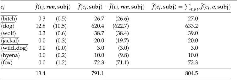
An example contingency table, based on counts obtained from a subset of the BNC using the system of Briscoe and Carroll, is given in Table 1. (Recall that the frequencies are estimated by distributing the count for a noun equally among the noun’s senses; this explains the fractional counts.) One column contains estimates of counts arising
Table 1
Contingency table for the children ofcaninein the subject position ofrun.
ci ˆf(ci,run,subj) ˆf(ci,subj)−ˆf(ci,run,subj) ˆf(ci,subj) =
v∈Vˆf(ci,v,subj)
bitch 0.3 (0.5) 26.7 (26.6) 27.0
dog 12.8 (10.5) 620.4 (622.7) 633.2
wolf 0.3 (0.6) 38.7 (38.4) 39.0
jackal 0.0 (0.3) 20.0 (19.7) 20.0
wild dog 0.0 (0.0) 3.0 (3.0) 3.0
hyena 0.0 (0.2) 10.0 (9.8) 10.0
fox 0.0 (1.2) 72.3 (71.1) 72.3
13.4 791.1 804.5
from concepts inciappearing in the subject position of the verbrun:ˆf(ci,run,subj). A second column presents estimates of counts arising from concepts in ci appearing in the subject position of a verb other thanrun. The figures in brackets are the expected values if the null hypothesis is true.
There is a choice of which statistic to use in conjunction with the chi-square test. The usual statistic encountered in textbooks is the Pearson chi-square statistic, de-notedX2:
X2=
i,j
(oij−eij)2 eij
(16)
where oij is the observed value for the cell in row i and column j, and eij is the corresponding expected value. An alternative statistic is the log-likelihood chi-square statistic, denotedG2:8
G2=2 i,j
oijloge oij eij
(17)
The two statistics have similar values when the counts in the contingency table are large (Agresti 1996). The statistics behave differently, however, when the table contains low counts, and, since corpus data are likely to lead to some low counts, the question of which statistic to use is an important one. Dunning (1993) argues for the use ofG2
rather thanX2, based on an analysis of the sampling distributions of G2 and X2, and
results obtained when using the statistics to acquire highly associated bigrams. We consider Dunning’s analysis at the end of this section, and the question of whether to useG2orX2will be discussed further there. For now, we continue with the discussion
of how the chi-square test is used in the generalization procedure.
For Table 1, the value ofG2 is 3.8, and the value ofX2is 2.5. Assuming a level of significance ofα=0.05, the critical value is 12.6 (for six degrees of freedom). Thus, for thisαvalue, the null hypothesis would not be rejected for either statistic, and the conclusion would be that there is no reason to suppose that p(run | canine,subj)is not a reasonable approximation ofp(run| dog,subj).
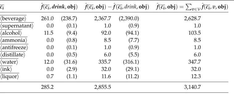
Table 2
Contingency table for the children ofliquidin the object position ofdrink.
ci ˆf(ci,drink,obj) ˆf(ci,obj)−ˆf(ci,drink,obj) ˆf(ci,obj) =
v∈Vˆf(ci,v,obj)
beverage 261.0 (238.7) 2,367.7 (2,390.0) 2,628.7
supernatant 0.0 (0.1) 1.0 (0.9) 1.0
alcohol 11.5 (9.4) 92.0 (94.1) 103.5
ammonia 0.0 (0.8) 8.5 (7.7) 8.5
antifreeze 0.0 (0.1) 1.0 (0.9) 1.0
distillate 0.0 (0.5) 6.0 (5.5) 6.0
water 12.0 (31.6) 335.7 (316.1) 347.7
ink 0.0 (2.9) 32.0 (29.1) 32.0
liquor 0.7 (1.1) 11.6 (11.2) 12.3
285.2 2,855.5 3,140.7
As a further example, Table 2 gives counts for the children ofliquidin the object position of drink. Again, the counts have been obtained from a subset of the BNC using the system of Briscoe and Carroll. Not all the sets dominated by the children of
liquidare shown, as some, such as sheep dip, never appear in the object position of a verb in the data. This example is designed to show a case in which the null hypothesis is rejected. The value of G2 for this table is 29.0, and the value of X2 is 21.2. So for G2, even if an αvalue as low as 0.0005 were being used (for which the critical value is 27.9 for eight degrees of freedom), the null hypothesis would still be rejected. For X2, the null hypothesis is rejected for α values greater than 0.005. This
seems reasonable, since the probabilities associated with the children of liquid and the object position of drink would be expected to show a lot of variation across the children.
A key question is how to select the appropriate value for α. One solution is to treatαas a parameter and set it empirically by taking a held-out test set and choosing the value of αthat maximizes performance on the relevant task. For example, Clark and Weir (2000) describes a prepositional phrase attachment algorithm that employs probability estimates obtained using the WordNet method described here. To set the value of α, the performance of the algorithm on a development set could be com-pared across different values of α, and the value that leads to the best performance could be chosen. Note that this approach sets no constraints on the value of α: The value could be as high as 0.995 or as low as 0.0005, depending on the particular application.
the counts they contain. The main problem with this test is that it is computationally expensive, especially for large contingency tables.
What we have found in practice is that applying the chi-square test to tables dom-inated by low counts tends to produce an insignificant result, and the null hypothesis is not rejected. The consequences of this for the generalization procedure are that low-count tables tend to result in the procedure moving up to the next node in the hierarchy. But given that the purpose of the generalization is to overcome the sparse-data problem, moving up a node is desirable, and therefore we do not modify the test for tables with low counts.
The final issue to consider is which chi-square statistic to use. Dunning (1993) argues for the use of G2 rather than X2, based on the claim that the sampling distri-bution of G2 approaches the true chi-square distribution quicker than the sampling
distribution of X2. However, Agresti (1996, page 34) makes the opposite claim: “The
sampling distributions of X2 and G2 get closer to chi-squared as the sample size n
increases. . . .The convergence is quicker forX2 thanG2.”
In addition, Pedersen (2001) questions whether one statistic should be preferred over the other for the bigram acquisition task and cites Cressie and Read (1984), who argue that there are some cases where the Pearson statistic is more reliable than the log-likelihood statistic. Finally, the results of the pseudo-disambiguation experiments presented in Section 7 are at least as good, if not better, when usingX2rather thanG2,
and so we conclude that the question of which statistic to use should be answered on a per application basis.
5. The Generalization Procedure
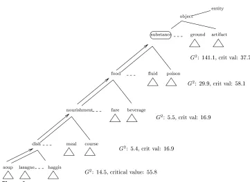
The procedure for finding a suitable class, c, to generalize concept c in position r of verbv works as follows. (We refer to c as the “similarity class” of cwith respect to v and r and the hypernymc as top(c,v,r), since the chosen hypernym sits at the “top” of the similarity class.) Initially, concept c is assigned to a variabletop. Then, by working up the hierarchy, successive hypernyms ofcare assigned totop, and this process continues until the probabilities associated with the sets of concepts dominated bytopand the siblings of topare significantly different. Once a node is reached that results in a significant result for the chi-square test, the procedure stops, and topis returned astop(c,v,r). In cases where a concept has more than one parent, the parent is chosen that results in the lowest value of the chi-square statistic, as this indicates the probabilities are the most similar. The settop(c,v,r)is the similarity class ofcfor verbvand position r. Figure 1 gives an algorithm for determiningtop(c,v,r).
Figure 2 gives an example of the procedure at work. Here, top(soup,stir,obj)is being determined. The example is based on data from a subset of the BNC, with 303 cases of an argument in the object position ofstir. TheG2statistic is used, together with an α value of 0.05. Initially, topis set to soup, and the probabilities corresponding to the children of dishare compared:p(stir| soup,obj),p(stir| lasagne,obj),p(stir|
haggis,obj), and so on for the rest of the children. The chi-square test results in aG2
value of 14.5, compared to a critical value of 55.8. SinceG2is less than the critical value,
the procedure moves up to the next node. This process continues until a significant result is obtained, which first occurs at substance when comparing the children of
object. Thussubstanceis the chosen level of generalization.
Algorithm top(c,v,r): top←c
sig result←false
commentparentmin gives lowestG2 value,G2min
whilenot sig result&top=rootdo
G2 min← ∞
for all parents oftopdo
calculateG2 for sets dominated by children ofparent
if G2<G2 min
then G2
min←G2
parentmin←parent
end
ifchi-square test forparentmin is significant
thensig result←true
elsemove up to next node:top←parentmin
[image:10.612.98.457.57.708.2]end returntop
Figure 1
An algorithm for determiningtop(c,v,r).
haggis lasagne
dish
nourishment
food
fare beverage
course meal
substance object
uid poison
artifact ground
entity
soup
G 2
: 14:5,criticalvalue: 55:8 G
2
: 5:4,critval: 16:9 G
2
: 5:5,critval: 16:9 G
2
: 29:9,critval: 58:1 G
2
[image:10.612.102.463.394.658.2]: 141:1,critval: 37:7
Figure 2
1997; Li and Abe 1998; Wagner 2000), the level of generalization is often determined for a small number of hand-picked verbs and the result compared with the researcher’s intuition about the most appropriate level for representing a selectional preference. According to this approach, if sandwich were chosen to represent hotdog in the object position of eat, this might be considered an undergeneralization, since food might be considered more appropriate. For this work we argue that such an evaluation is not appropriate; since the purpose of this work is probability estimation, the most appropriate level is the one that leads to the most accurate estimate, and this may or may not agree with intuition. Furthermore, we show in Section 7 that to generalize unnecessarily can be harmful for some tasks: If we already have lots of data regarding
sandwich, why generalize any higher? Thus the purpose of this section is not to show that the acquired levels are “correct,” but simply to show how the levels vary withα
and the sample size.
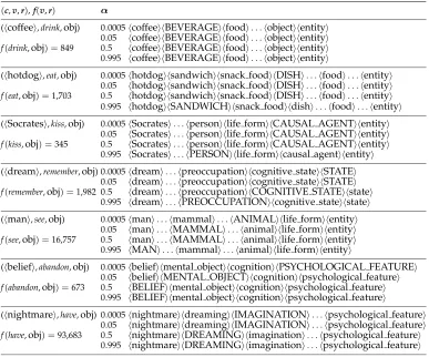
To show how the level of generalization varies with changes in α, top(c,v,obj)
was determined for a number of hand-picked(c,v,obj)triples over a range of values forα. The triples were chosen to give a range of strongly and weakly selecting verbs and a range of verb frequencies. The data were again extracted from a subset of the BNC using the system of Briscoe and Carroll (1997), and theG2 statistic was used in
the chi-square test. The results are shown in Table 3. The number of times the verb occurred with some object is also given in the table.
The results suggest that the generalization level becomes more specific as α in-creases. This is to be expected, since, given a contingency table chosen at random, a higher value ofαis more likely to lead to a significant result than a lower value ofα. We also see that, for some cases, the value ofαhas little effect on the level. We would expect there to be less change in the level of generalization for strongly selecting verbs, such as drink and eat, and a greater range of levels for weakly selecting verbs such as see. This is because any significant difference in probabilities is likely to be more marked for a strongly selecting verb, and likely to be significant over a wider range of αvalues. The table only provides anecdotal evidence, but provides some support to this argument.
To investigate more generally how the level of generalization varies with changes inα, and also with changes in sample size, we took 6, 000(c,v,obj)triples and calcu-lated the difference in depth betweencandtop(c,v,r)for each triple. The 6, 000 triples were taken from the first experimental test set described in Section 7, and the train-ing data from this experiment were used to provide the counts. (The test set contains nouns, rather than noun senses, and so the sense of the noun that is most probable given the verb and object slot was used.) An average difference in depth was then calculated. To give an example of how the difference in depth was calculated, sup-pose dog generalized toplacental mammal via canine and carnivore; in this case the difference would be three.
Table 3
Example levels of generalization for different values ofα.
(c,v,r),f(v,r) α
(coffee,drink,obj) 0.0005coffeeBEVERAGEfood. . .objectentity
0.05 coffeeBEVERAGEfood. . .objectentity f(drink,obj) =849 0.5 coffeeBEVERAGEfood. . .objectentity
0.995 coffeeBEVERAGEfood. . .objectentity
(hotdog,eat,obj) 0.0005hotdogsandwichsnack foodDISH. . .food. . .entity
0.05 hotdogsandwichsnack foodDISH. . .food. . .entity f(eat,obj) =1,703 0.5 hotdogsandwichsnack foodDISH. . .food. . .entity
0.995 hotdogSANDWICHsnack fooddish. . .food. . .entity
(Socrates,kiss,obj) 0.0005Socrates. . .personlife formCAUSAL AGENTentity
0.05 Socrates. . .personlife formCAUSAL AGENTentity f(kiss,obj) =345 0.5 Socrates. . .personlife formCAUSAL AGENTentity
0.995 Socrates. . .PERSONlife formcausal agententity
(dream,remember,obj) 0.0005dream. . .preoccupationcognitive stateSTATE
0.05 dream. . .preoccupationcognitive stateSTATE f(remember,obj) =1,982 0.5 dream. . .preoccupationCOGNITIVE STATEstate
0.995 dream. . .PREOCCUPATIONcognitive statestate
(man,see,obj) 0.0005man. . .mammal. . .ANIMALlife formentity
0.05 man. . .MAMMAL. . .animallife formentity f(see,obj) =16,757 0.5 man. . .MAMMAL. . .animallife formentity
0.995 MAN. . .mammal. . .animallife formentity
(belief,abandon,obj) 0.0005beliefmental objectcognitionPSYCHOLOGICAL FEATURE 0.05 beliefMENTAL OBJECTcognitionpsychological feature
f(abandon,obj) =673 0.5 BELIEFmental objectcognitionpsychological feature 0.995 BELIEFmental objectcognitionpsychological feature
(nightmare,have,obj) 0.0005nightmaredreamingIMAGINATION. . .psychological feature
0.05 nightmaredreamingIMAGINATION. . .psychological feature f(have,obj) =93,683 0.5 nightmareDREAMINGimagination. . .psychological feature
[image:12.612.102.492.505.569.2]0.995 nightmareDREAMINGimagination. . .psychological feature Note:The selected level is shown in upper case.
Table 4
Extent of generalization for different values ofαand sample sizes.
α 100% 50% 10% 1%
0.0005 3.3 3.9 5.0 5.6 0.05 2.8 3.5 4.6 5.6 0.5 2.1 2.9 4.1 5.4 0.995 1.2 1.5 2.6 3.9
size. Again, this is to be expected, since any difference in probability estimates is less likely to be significant for tables with low counts.
6. Alternative Class-Based Estimation Methods
The first alternative uses the “association score,” which is a measure of how well a set of concepts,C, satisfies the selectional preferences of a verb,v, for an argument position,r:9
A(C,v,r) =p(C|v,r)log2 p(C|v,r)
p(C|r) (18)
An estimate of the association score,Aˆ(C,v,r), can be obtained using relative frequency
estimates of the probabilities. The key question is how to determine a suitable level of generalization for conceptc, or, alternatively, how to find a suitable class to represent concept c (assuming the choice is from those classes that contain all concepts dom-inated by some hypernym of c). Resnik’s solution to this problem (which he neatly refers to as the “vertical-ambiguity” problem) is to choose the class that maximizes the association score.
It is not clear that the class with the highest association score is always the most appropriate level of generalization. For example, this approach does not always gen-eralize appropriately for arguments that are negativelyassociated with some verb. To see why, consider the problem of deciding how well the conceptlocationsatisfies the preferences of the verbeatfor its object. Since locations are not the kinds of things that are typically eaten, a suitable level of generalization would correspond to a class that has a low association score with respect toeat. However,locationis a kind ofentity in WordNet,10 and choosing the class with the highest association score is likely to produceentityas the chosen class. This is a problem, because the association score ofentitywith respect toeatmay be too high to reflect the fact thatlocationis a very unlikely object of the verb.
Note that the solution to the vertical-ambiguity problem presented in the previous sections is able to generalize appropriately in such cases. Continuing with the eat
location example, our generalization procedure is unlikely to get as high as entity (assuming a reasonable number of examples of eat in the training data), since the probabilities corresponding to the daughters ofentityare likely to be very different with respect to the object position of eat.
The second alternative uses the minimum description length (MDL) principle. Li and Abe use MDL to select a set of classes from a hierarchy, together with their associated probabilities, to represent the selectional preferences of a particular verb. The preferences and class-based probabilities are then used to estimate probabilities of the formp(n|v,r), wheren is a noun,v is a verb, andris an argument slot.
Li and Abe’s application of MDL requires the hierarchy to be in the form of a thesaurus, in which each leaf node represents a noun and internal nodes represent the class of nouns that the node dominates. The hierarchy is also assumed to be in the form of a tree. The class-based models consist of a partition of the set of nouns (leaf nodes) and a probability associated with each class in the partition. The probabilities are the conditional probabilities of each class, given the relevant verb and argument position. Li and Abe refer to such a partition as a “cut” and the cut together with the probabilities as a “tree cut model.” The probabilities of the classes in a cut,Γ, satisfy the following constraint:
C∈Γ
p(C|v,r) =1 (19)
9 The definition used here is that given by Ribas (1995).
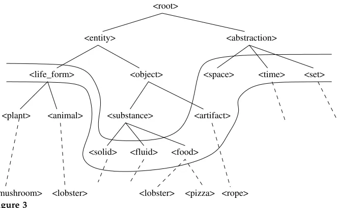
<abstraction>
<life_form>
<plant>
<object> <entity>
<substance>
<set> <root>
<mushroom>
<artifact>
<rope> <food>
<pizza> <lobster>
<fluid> <solid>
<animal>
<lobster>
[image:14.612.112.443.85.290.2]<time> <space>
Figure 3
Possible cut returned by MDL.
In order to determine the probability of a noun, the probability of a class is assumed to be distributed uniformly among the members of that class:
p(n|v,r) = 1
|C| p(C|v,r) for all n∈C (20)
Since WordNet is a hierarchy with noun senses, rather than nouns, at the nodes, Li and Abe deal with the issue of word sense ambiguity using the method described in Section 3, by dividing the count for a noun equally among the concepts whose synsets contain the noun. Also, since WordNet is a DAG, Li and Abe turn WordNet into a tree by copying each subgraph with multiple parents. And so that each noun in the data appears (in a synset) at a leaf node, Li and Abe remove those parts of the hierarchy dominated by a noun in the data (but only for that instance of WordNet corresponding to the relevant verb).
An example cut showing part of the WordNet hierarchy is shown in Figure 3 (based on an example from Li and Abe [1998]; the dashed lines indicate parts of the hierarchy that are not shown in the diagram). This is a possible cut for the object position of the verbeat, and the cut consists of the following classes:life form,solid,fluid,food,
artifact,space,time,set. (The particular choice of classes for the cut in this example is not too important; the example is designed to show how probabilities of senses are estimated from class probabilities.) Since the class in the cut containingpizzaisfood, the probability p(pizza | eat,obj) would be estimated as p(food | eat,obj)/|food|. Similarly, since the class in the cut containingmushroomislife form, the probability p(mushroom |eat,obj)would be estimated asp(life form |eat,obj)/|life form|.
term and denotes the number of bits required to encode the model. The fit to the data is measured using the data description length, which is the number of bits required to encode the data (relative to the model). The overall description length is the sum of the model description length and the data description length, and the MDL principle is to select the model with the shortest description length.
We used McCarthy’s (2000) implementation of MDL. So that every noun is repre-sented at a leaf node, McCarthy does not remove parts of the hierarchy, as Li and Abe do, but instead creates new leaf nodes for each synset at an internal node. McCarthy also does not transform WordNet into a tree, which is strictly required for Li and Abe’s application of MDL. This did create a problem with overgeneralization: Many of the cuts returned by MDL were overgeneralizing at the entity node. The reason is thatperson, which is close toentityand dominated by entity, has two parents:
life form and causal agent. This DAG-like property was responsible for the over-generalization, and so we removed the link between personand causal agent. This appeared to solve the problem, and the results presented later for the average degree of generalization do not show an overgeneralization compared with those given in Li and Abe (1998).
7. Pseudo-Disambiguation Experiments
The task we used to compare the class-based estimation techniques is a decision task previously used by Pereira, Tishby, and Lee (1993) and Rooth et al. (1999). The task is to decide which of two verbs,v and v, is more likely to take a given noun,n, as an object. The test and training data were obtained as follows. A number of verb–direct object pairs were extracted from a subset of the BNC, using the system of Briscoe and Carroll. All those pairs containing a noun not in WordNet were removed, and each verb and argument was lemmatized. This resulted in a data set of around 1.3 million
(v,n)pairs.
To form a test set, 3,000 of these pairs were randomly selected such that each selected pair contained a fairly frequent verb. (Following Pereira, Tishby, and Lee, only those verbs that occurred between 500 and 5,000 times in the data were considered.) Each instance of a selected pair was then deleted from the data to ensure that the test data were unseen. The remaining pairs formed the training data. To complete the test set, a further fairly frequent verb, v, was randomly chosen for each (v,n) pair. The random choice was made according to the verb’s frequency in the original data set, subject to the condition that the pair (v,n)did not occur in the training data. Given the set of (v,n,v)triples, the task is to decide whether (v,n) or(v,n) is the correct pair.11
We acknowledge that the task is somewhat artificial, but pseudo-disambiguation tasks of this kind are becoming popular in statistical NLP because of the ease with which training and test data can be created. We also feel that the pseudo-disambig-uation task is useful for evaluating the different estimation methods, since it directly addresses the question of how likely a particular predicate is to take a given noun as an argument. An evaluation using a PP attachment task was attempted in Clark and Weir (2000), but the evaluation was limited by the relatively small size of the Penn Treebank.
Table 5
Results for the pseudo-disambiguation task.
Generalization technique % correct av.gen. sd.gen.
Similarity class
α=0.0005 73.8 3.3 2.0
α=0.05 73.4 2.8 1.9
α=0.3 73.0 2.4 1.8
α=0.75 73.9 1.9 1.6
α=0.995 73.8 1.2 1.2
Low class 73.6 0.9 1.0
MDL 68.3 4.1 1.9
Assoc 63.9 4.2 2.1
Note:av.gen. is the average number of generalized levels; sd.gen. is the standard deviation.
Using our approach, the disambiguation decision for each(v,n,v)triple was made according to the following procedure:
if max
c∈cn(n)psc
(c|v,obj) > max c∈cn(n)psc
(c|v,obj)
then choose(v,n)
else if max
c∈cn(n)psc(c|v
,obj) > max
c∈cn(n)psc(c|v,obj)
then choose(v,n)
else choose at random
If n has more than one sense, the sense is chosen that maximizes the relevant prob-ability estimate; this explains the maximization over cn(n). The probability estimates were obtained using our class-based method, and the G2 statistic was used for the
chi-square test. This procedure was also used for the MDL alternative, but using the MDL method to estimate the probabilities.
Using the association score for each test triple, the decision was made according to the following procedure:
if max
c∈cn(n) cmax∈h(c) ˆ
A(c,v,obj) > max
c∈cn(n) cmax∈h(c) ˆ
A(c,v,obj)
then choose(v,n)
else if max
c∈cn(n) cmax∈h(c) ˆ
A(c,v,obj) > max
c∈cn(n) cmax∈h(c) ˆ
A(c,v,obj)
then choose(v,n)
else choose at random
We useh(c)to denote the set consisting of the hypernyms ofc. The inner maximization is overh(c), assumingcis the chosen sense ofn, which corresponds to Resnik’s method of choosing a set to representc. The outer maximization is over the senses ofn,cn(n), which determines the sense ofnby choosing the sense that maximizes the association score.
Table 6
Results for the pseudo-disambiguation task with one-fifth training data.
Generalization technique % correct av.gen. sd.gen.
Similarity class
α=0.0005 66.7 4.5 1.9
α=0.05 68.4 4.1 1.9
α=0.3 70.2 3.7 1.9
α=0.75 72.3 3.0 1.9
α=0.995 72.4 1.9 1.6
Low class 71.9 1.1 1.1
MDL 62.9 4.7 1.9
Assoc 62.6 4.1 2.0
Note:av.gen. is the average number of generalized levels; sd.gen. is the standard deviation.
to as “Assoc.” The results are given for a range ofαvalues and demonstrate clearly that the performance of similarity class varies little with changes inα and that similarity class outperforms both MDL and Assoc.12
We also give a score for our approach using a simple generalization procedure, which we call “low class.” The procedure is to select the first class that has a count greater than zero (relative to the verb and argument position), which is likely to return a low level of generalization, on the whole. The results show that our generalization technique only narrowly outperforms the simple alternative. Note that, although low class is based on a very simple generalization method, the estimation method is still using our class-based technique, by applying Bayes’ theorem and conditioning on a class, as described in Section 3; the difference is in how the class is chosen.
To investigate the results, we calculated the average number of generalized levels for each approach. The number of generalized levels for a concept c (relative to a verb v and argument positionr) is the difference in depth between cand top(c,v,r), as explained in Section 5. For each test case, the number of generalized levels for both verbs, v and v, was calculated, but only for the chosen sense of n. The results are given in the third column of Table 5 and demonstrate clearly that both MDL and Assoc are generalizing to a greater extent than similarity class. (The fourth column gives a standard deviation figure.) These results suggest that MDL and Assoc are overgeneralizing, at least for the purposes of this task.
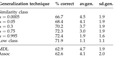
To investigate why the value forαhad no impact on the results, we repeated the experiment, but with one fifth of the data. A new data set was created by taking every fifth pair of the original 1.3 million pairs. A test set of 3,000 triples was created from this new data set, as before, but this time only verbs that occurred between 100 and 1,000 times were considered. The results using these test and training data are given in Table 6.
These results show a variation in performance across values forα, with an opti-mal performance whenαis around 0.75. (Of course, in practice, the value forαwould need to be optimized on a held-out set.) But even with this variation, similarity class is still outperforming MDL and Assoc across the whole range ofαvalues. Note that the
Table 7
Disambiguation results forG2andX2.
αvalue % correct (G2) % correct (X2)
0.0005 73.8 (3.3) 74.1 (3.0)
0.05 73.4 (2.8) 73.8 (2.5)
0.3 73.0 (2.4) 74.1 (2.2)
0.75 73.9 (1.9) 74.3 (1.8)
0.995 73.8 (1.2) 73.3 (1.2)
αvalues corresponding to the lowest scores lead to a significant amount of general-ization, which provides additional evidence that MDL and Assoc are overgeneralizing for this task. The low-class method scores highly for this data set also, but given that the task is one that apparently favors a low level of generalization, the high score is not too surprising.
As a final experiment, we compared the task performance using theX2, rather than G2, statistic in the chi-square test. The results are given in Table 7 for the complete data set.13 The figures in brackets give the average number of generalized levels. The X2 statistic is performing at least as well as G2, and the results show that the
average level of generalization is slightly higher forG2thanX2. This suggests a possible
explanation for the results presented here and those in Dunning (1993): that the X2
statistic provides a less conservative test when counts in the contingency table are low. (By a conservative test we mean one in which the null hypothesis is not easily rejected.) A less conservative test is better suited to the pseudo-disambiguation task, since it results in a lower level of generalization, on the whole, which is good for this task. In contrast, the task that Dunning considers, the discovery of bigrams, is better served by a more conservative test.
8. Conclusion
We have presented a class-based estimation method that incorporates a procedure for finding a suitable level of generalization in WordNet. This method has been shown to provide superior performance on a pseudo-disambiguation task, compared with two alternative approaches. An analysis of the results has shown that the other approaches appear to be overgeneralizing, at least for this task. One of the features of the gener-alization procedure is the way that α, the level of significance in the chi-square test, is treated as a parameter. This allows some control over the extent of generalization, which can be tailored to particular tasks. We have also shown that the task perfor-mance is at least as good when using the Pearson chi-square statistic as when using the log-likelihood chi-square statistic.
There are a number of ways in which this work could be extended. One possibility would be to use all the classes dominated by the hypernyms of a concept, rather than just one, to estimate the probability of the concept. An estimate would be obtained for each hypernym, and the estimates combined in a linear interpolation. An approach similar to this is taken by Bikel (2000), in the context of statistical parsing.
There is still room for investigation of the hidden-data problem when data are used that have not been sense disambiguated. In this article, a very simple approach is taken,
which is to split the count for a noun evenly among the noun’s senses. Abney and Light (1999) have tried a more motivated approach, using the expectation maximization algorithm, but with little success. The approach described in Clark and Weir (1999) is shown in Clark (2001) to have some impact on the pseudo-disambiguation task, but only with certain values of theαparameter, and ultimately does not improve on the best performance.
Finally, an issue that has not been much addressed in the literature (except by Li and Abe [1996]) is how the accuracy of class-based estimation techniques compare when automatically acquired classes, as opposed to the manually created classes from WordNet, are used. The pseudo-disambiguation task described here has also been used to evaluate clustering algorithms (Pereira, Tishby, and Lee, 1993; Rooth et al., 1999), but with different data, and so it is difficult to compare the results. A related issue is how the structure of WordNet affects the accuracy of the probability estimates. We have taken the structure of the hierarchy for granted, without any analysis, but it may be that an alternative design could be more conducive to probability estimation.
Acknowledgments
This article is an extended and updated version of a paper that appeared in the proceedings of NAACL 2001. The work on which it is based was carried out while the first author was a D.Phil. student at the University of Sussex and was supported by an EPSRC studentship. We would like to thank Diana McCarthy for suggesting the pseudo-disambiguation task and providing the MDL software, John Carroll for supplying the data, and Ted Briscoe, Geoff Sampson, Gerald Gazdar, Bill Keller, Ted Pedersen, and the anonymous reviewers for their helpful comments. We would also like to thank Ted Briscoe for presenting an earlier version of this article on our behalf at NAACL 2001.
References
Abney, Steven P. and Marc Light. 1999. Hiding a semantic hierarchy in a Markov model. InProceedings of the ACL Workshop on Unsupervised Learning in Natural Language Processing, University of Maryland, College Park, pages 1–8. Agirre, Eneko and David Martinez. 2001.
Learning class-to-class selectional preferences. InProceedings of the Fifth ACL Workshop on Computational Language Learning, Toulouse, France, pages 15–22. Agresti, Alan. 1996.An Introduction to
Categorical Data Analysis. Wiley. Bikel, Daniel M. 2000. A statistical model
for parsing and word-sense
disambiguation. InProceedings of the Joint SIGDAT Conference on Empirical Methods in Natural Language Processing and Very Large Corpora, pages 155–163, Hong Kong. Briscoe, Ted and John Carroll. 1997.
Automatic extraction of subcategorization from corpora. InProceedings of the Fifth ACL Conference on Applied Natural Language Processing, pages 356–363, Washington, DC.
Church, Kenneth W. and Patrick Hanks. 1990. Word association norms, mutual information, and lexicography.
Computational Linguistics, 16(1):22–29. Ciaramita, Massimiliano and Mark Johnson.
2000. Explaining away ambiguity: Learning verb selectional preference with Bayesian networks. InProceedings of the 18th International Conference on
Computational Linguistics, pages 187–193, Saarbrucken, Germany.
Clark, Stephen. 2001.Class-Based Statistical Models for Lexical Knowledge Acquisition. Ph.D. dissertation, University of Sussex. Clark, Stephen and David Weir. 1999. An
iterative approach to estimating
frequencies over a semantic hierarchy. In
Proceedings of the Joint SIGDAT Conference on Empirical Methods in Natural Language Processing and Very Large Corpora, pages 258–265, University of Maryland, College Park.
Clark, Stephen and David Weir. 2000. A class-based probabilistic approach to structural disambiguation. InProceedings of the 18th International Conference on Computational Linguistics, pages 194–200, Saarbrucken, Germany.
Clark, Stephen and David Weir. 2001. Class-based probability estimation using a semantic hierarchy. InProceedings of the Second Meeting of the North American Chapter of the Association for Computational Linguistics, pages 95–102, Pittsburgh. Cressie, Noel A. C. and Timothy R. C. Read.
Journal of the Royal Statistics Society Series B, 46:440–464.
Dunning, Ted. 1993. Accurate methods for the statistics of surprise and coincidence.
Computational Linguistics, 19(1):61–74. Fellbaum, Christiane, editor. 1998.WordNet:
An Electronic Lexical Database. MIT Press. Li, Hang and Naoki Abe. 1996. Clustering
words with the MDL principle. In
Proceedings of the 16th International Conference on Computational Linguistics, pages 4–9, Copenhagen, Denmark. Li, Hang and Naoki Abe. 1998. Generalizing
case frames using a thesaurus and the MDL principle.Computational Linguistics, 24(2):217–244.
McCarthy, Diana. 1997. Word sense disambiguation for acquisition of selectional preferences. InProceedings of the ACL/EACL Workshop on Automatic Information Extraction and Building of Lexical Semantic Resources for NLP Applications, pages 52–61, Madrid.
McCarthy, Diana. 2000. Using semantic preferences to identify verbal participation in role switching. In
Proceedings of the First Conference of the North American Chapter of the Association for Computational Linguistics, pages 256–263, Seattle.
Miller, George A. 1998. Nouns in WordNet. In Christiane Fellbaum, editor,WordNet: An Electronic Lexical Database. MIT Press, pages 23–46.
Pedersen, Ted. 1996. Fishing for exactness. InProceedings of the South-Central SAS Users Group Conference, Austin, pages 188–200. Pedersen, Ted. 2001. A decision tree of
bigrams is an accurate predictor of word sense. InProceedings of the Second Meeting of the North American Chapter of the Association for Computational Linguistics, pages 79–86, Pittsburgh.
Pereira, Fernando, Naftali Tishby, and Lillian Lee. 1993. Distributional clustering of English words. InProceedings of the 31st Annual Meeting of the Association for Computational Linguistics, pages 183–190, Columbus, OH.
Resnik, Philip. 1993.Selection and Information: A Class-Based Approach to Lexical Relationships. Ph.D. dissertation, University of Pennsylvania.
Resnik, Philip. 1998. WordNet and class-based probabilities. In Christiane Fellbaum, editor,WordNet: An Electronic Lexical Database. MIT Press, pages 239–263. Ribas, Francesc. 1995. On learning more
appropriate selectional restrictions. In
Proceedings of the Seventh Conference of the European Chapter of the Association for Computational Linguistics, pages 112–118, Dublin.
Rooth, Mats, Stefan Riezler, Detlef Prescher, Glenn Carroll, and Franz Beil. 1999. Inducing a semantically annotated lexicon via EM-based clustering. InProceedings of the 37th Annual Meeting of the Association for Computational Linguistics, pages 104–111, University of Maryland, College Park. Wagner, Andreas. 2000. Enriching a lexical
semantic net with selectional preferences by means of statistical corpus analysis. In