1D Modeling of Controlled-Source Electromagnetic (CSEM) Data using Finite Element Method for Hydrocarbon Detection in Shallow Water

1D Modeling of Controlled-Source Electromagnetic

(CSEM) Data using Finite Element Method for

Hydrocarbon Detection in Shallow Water

Noor Hazrin Hany Mohamad Hanif, Nazabat Hussain, Norashikin Yahya, Hanita Daud, Noorhana Yahya, Mohd Noh

Karsiti

Abstract—The utilization of controlled-source electromagnetic (CSEM) method has gained tremendous interest among the offshore exploration community in these recent years. This application is especially significant in detecting hydrocarbon in shallow waters. The success of this method in the search of oil and gas reservoirs is due to the fact that hydrocarbon-saturated-reservoirs are characterized by very high resistivity, while the surrounding saline water formations are very conductive. Through these characteristics, the resistivity of the sea subsurface could be mapped via the electric and magnetic field data collected in CSEM survey. Modeling is done using finite element method, which is a flexible computational method that utilizes unstructured grids that can readily conform to irregular boundaries such as seafloor topography. This paper highlights the application of the finite element method in processing the CSEM data to produce the 1D model of hydrocarbon reservoir. The CSEM data is gathered through experiments using a 90-cm deep water tank that has been designed to represent the actual system of seabed logging. The obtained results show that the modeling method is capable to become an alternative solution in hydrocarbon detection.

Keywords-Controlled Source Electromagnetic (CSEM), Finite Element, Hydrocarbon detection

I. INTRODUCTION

The use of controlled-source electromagnetic (CSEM) method to estimate the spatial variation of subsurface electrical resistivity has gain significant interest among the offshore exploration community [1-3]. The success of the method in the search of oil and gas reservoirs is based on the fundamental fact that hydrocarbon-saturated-reservoirs are characterized by very high resistivity, while the surrounding saline water formations are very conductive. The CSEM technique as illustrated in Figure 1 uses a mobile horizontal electric dipole (HED) source and an array

Manuscript received January 14, 2011, revised February 1, 2011. This work was funded by the Malaysian Ministry of Higher Education (MOHE) under the Fundamental Research Grant Scheme (FRGS).

Noor Hazrin Hany Mohamad Hanif and Mohd Noh Karsiti are with the Electrical & Electronic Engineering Department of Universiti Teknologi PETRONAS, Malaysia. (phone: 605-3687866; e-mail:

[email protected], [email protected]).

Nazabat Hussain and Norashikin Yahya are Masters and PhD students with the Electrical & Electronic Engineering Department of Universiti Teknologi PETRONAS, Malaysia.

Hanita Daud and Noorhana Yahya are with the Fundamental and Applied Sciences Department, University Teknologi PETRONAS, Malaysia.

of electric, plus on occasion magnetic, dipole field receivers located on the seafloor. The HED source emits a low frequency electromagnetic signal (usually from 0.1Hz to 10 Hz) that diffuses outward through both sea water and through the sea subsurface formations.

[image:1.612.319.562.422.588.2]

Due to the lower conductivity of sea subsurface formations (less than 1 S/m), the diffusion rate of EM signals through the seafloor will be higher than that directly through the sea. As a result, at a suitable horizontal range, the electric field measured at the seafloor by a receiving electric dipole can be dominated by the response from the subsea formations. The measurements of both the amplitude and phase of the receiving signals can then in principle be used to determine the subsurface geology, especially if it contains a higher resistivity hydrocarbon filled layer. In-depth historical context of CSEM method and the development from academic and industry is being covered in works by [4].

Figure 1. Schematic representation of the horizontal electric dipole-dipole marine CSEM method [4].

FEM is the most suitable technique in modeling electromagnetic waves for hydrocarbon explorations as it could be easily conformed to irregular wave problems as compared to FDM, which could only compute in regular rectangular shapes. In principle, finite difference and finite element methods are capable in modeling arbitrary sources and three dimensional (3D) structures. 3D methods using staggered-grid finite differences [7, 8] allow for multidimensional modeling of heterogeneous structures, yet these methods are bound by structural grid. MOM is also less preferred for this problem as it yields complicated derivation of governing equations as compared to FEM [9].

Development of higher-dimensional finite element models such as shown by works of [10] highlights a high possibility that it could be used for inversion of multidimensional data. Through this inversion, the actual location of hydrocarbon reservoir could be determined.

[image:2.612.307.561.56.191.2]

Although higher-dimensional models may provide better representation of actual models, the 1D model has significant contribution for the exploration works as well. It is most useful when collected data sets in the marine environment are insufficient to be processed in multidimensional interpretation. It could also be utilized for comparison purposes against the multidimensional methods. On top of that, due to its simplicity, the 1D model provides faster computations and requires less memory space [11]. Examples on the capability of 1D model for hydrocarbon detection are shown by works of [11, 12].

II. GEOLOGICAL MODEL

[image:2.612.319.552.288.619.2]

The 3D model of a seabed logging system, utilized for this work, is as shown in Figure 2. The model is a 90cm deep water tank, with length and width of 180 cm and 90 cm respectively. Three receivers are located 28 cm from the bottom of the tank, completely immersed in the water. One transmitter is mounted above the tank, to be manually moved from one end of the tank to another. A packet of cooking oil that represents hydrocarbon source is placed at the bottom of the tank. Figure 3 shows the 2D geological model of the water tank.

Figure 2: 3-Dimensional water tank dimensions for the interpretations of EM-field in Marine CSEM survey for

seabed logging

Figure 3: 2-Dimensional water tank dimensions for the interpretations of EM-field in Marine CSEM survey for

seabed logging

[image:2.612.318.552.289.618.2]

Complete model parameters of the system are tabulated in Table I. The permittivity values of sediments and water are taken from [13].

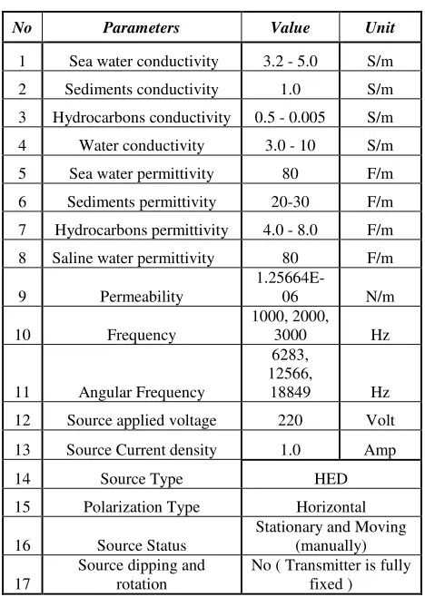
TABLE I. MODEL PARAMETERS OF THE WATER TANK

No Parameters Value Unit

1 Sea water conductivity 3.2 - 5.0 S/m 2 Sediments conductivity 1.0 S/m 3 Hydrocarbons conductivity 0.5 - 0.005 S/m 4 Water conductivity 3.0 - 10 S/m 5 Sea water permittivity 80 F/m 6 Sediments permittivity 20-30 F/m 7 Hydrocarbons permittivity 4.0 - 8.0 F/m 8 Saline water permittivity 80 F/m

9 Permeability

1.25664E-06 N/m

10 Frequency

1000, 2000, 3000 Hz

11 Angular Frequency

6283, 12566,

18849 Hz 12 Source applied voltage 220 Volt

13 Source Current density 1.0 Amp

14 Source Type HED

15 Polarization Type Horizontal

16 Source Status

Stationary and Moving (manually)

17

Source dipping and rotation

No ( Transmitter is fully fixed )

III. APPROACH

[image:2.612.54.292.506.639.2]

Figure 4: Simplified 1-Dimensional water tank dimensions of the water tank

The basis of this approach is the electromagnetic signals by the electric dipole source and the mobile electric field receivers. In practical deepwater hydrocarbon exploration, low frequencies (up until 1 kHz) are utilized for signal transmission, due to the fact that low frequencies provide farther penetration. However, as this work deals with a very shallow water (less than 1m), higher frequencies are utilized to allow signal penetration from the stationary transmitter above the water tank, passing through overlaying water and towards the receiver.

IV. GOVERNING EQUATIONS FOR 1-DIMENSIONAL GEOLOGICAL MODEL

The partial differential equation for electric field (E), in relation to current source (J) for 1D is as shown as follows:

S

J

i

i

µσω

Ε

−

µω

−

Ε

µεω

=

Ε

×

∇

×

∇

2 (1)

The vector identity from (1) is further formulated to the following equations:

∇

×

∇

×

Ε

=

∇

(

∇

⋅

Ε

)

−

∇

2

Ε

(2)

S

J

i

i

µσω

Ε

−

µω

−

Ε

µεω

=

Ε

∇

−

Ε

⋅

∇

∇

(

)

2 2 (3)

₋

_∇

2

_Ε

₌

_µεω

2

_Ε

v

₋

_i

_µσω

_Ε

v

₋

_i

_µω

_J

S ₍₄₎

S

J

i

i

µεω

+

µσω

Ε

−

+

µω

−

=

Ε

∇

2

(

2

)

₍₅₎

If there is no source current, equation (5) will become

∇

2

Ε

=

−

(

_i

µεω

2

+

µσω

)

Ε

v

₍₆₎ 2

(

2

)

0

=

Ε

µσω

+

µεω

+

Ε

∇

i

v

(7)

The partial differential equation for magnetic field (H), is as follows:

S

J

i

µσω

Η

+

∇

×

−

Η

µεω

=

Η

×

∇

×

∇

v

2

v

v

(8)

S

J

i

µσω

Η

+

∇

×

−

Η

µεω

=

Η

∇

−

2

v

2

v

v

(9)

The differential equations for the 1D model could be further developed to the following equations:

2 ₀ 2 2 = Ε + Ζ ∂ Ε

∂v v

k (10)

S

J i k Ε = µω +

Ζ ∂

Ε

∂v v

2 2 2 (11) S J k Η =∇× +

Ζ ∂

Η

∂v v

2 2 2 (12) 2 ₀ 2 2 = Η + Ζ ∂ Η Ε

∂vv v

k (13)

V. FINITE ELEMENT SOLUTION TO CSEMMODELING In the construction of a finite element approximation for boundary value problem, equations (1) and (8) are expressed in variational or weak form [14]. The weak form requires the equality of both sides of (1) and (8) in the inner product sense. Consider a complex Hilbert space L₂(V) of the vector functions determined in the modeling region V and integrable

in V . The L₂(V) inner product of two complex vector

fields x and y is defined as

dv

V V

L ( .) ( )

) ,

( _{( )} *

2 x r y r

y

x =

∫∫∫

. (14)

Here, the region V in which calculations are to be made is

divided into elements.

The approximate solution of the electromagnetic field equations are in the form of

, ) ( ) ( 1

∑

= ≈ N n n n

a v r r

E (15a)

_{( ) ( ),} 1

∑

= ≈ N n n n

b v r r

H (15b)

where a_n,b_n(n=1,2, ..,.N) are the scalar coefficients of the expansions. The second order electric or magnetic field equations (1) and (8) can be written in operator form as

s

i i

L− ωµσ)E= ωµJ

( (16a)

s

i

L− )H=∇×J

( ωµσ (16b) where L is the second order differential operators given

by,L=∇×(∇×).

These equations were programmed and simulated in the MATLAB environment to investigate the effect of frequency variations to the electric field and phase angle between the receiver-transmitter separations for different layers of hydrocarbons.

VI. SIMULATED RESULTS

(a)

0 0.1 0.2 0.3 0.4 0.5 0.6 0.7 0.8 0.9

-5.44 -5.42 -5.4 -5.38 -5.36 -5.34 -5.32 -5.3

Source-receiver separation (m)

L

o

g

1

0

(E

le

c

tr

ic

f

ie

ld

(

V

/A

m

2)

0.05 HC thickness 0.1 HC thickness 0.15 HC thickness

[image:4.612.51.266.58.426.2]

(b)

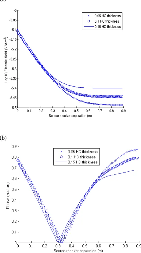
Figure 4: The response of a 1D model comprising 0.05 m, 0.1 m and 0.05 m thick hydrocarbon layer for varied distances between receiver and transmitter for 1 kHz. (a) The electric field strength (b) Phase angle

(a)

0 0.1 0.2 0.3 0.4 0.5 0.6 0.7 0.8 0.9

-5.5 -5.45 -5.4 -5.35 -5.3 -5.25 -5.2

Source-receiver separation (m)

L

o

g

1

0

(E

le

c

tr

ic

f

ie

ld

(

V

/A

m

2)

0.05 HC thickness 0.1 HC thickness 0.15 HC thickness

[image:4.612.330.545.63.234.2]

(b)

Figure 5: The response of a 1D model comprising 0.05 m, 0.1 m and 0.05 m thick hydrocarbon layer for varied distances between receiver and transmitter for 2 kHz. (a) The electric field strength (b) Phase angle

(a)

0 0.1 0.2 0.3 0.4 0.5 0.6 0.7 0.8 0.9

-5.5 -5.45 -5.4 -5.35 -5.3 -5.25 -5.2 -5.15 -5.1 -5.05 -5

Source-receiver separation (m)

L

o

g

1

0

(E

le

c

tr

ic

f

ie

ld

(

V

/A

m

2)

0.05 HC thickness 0.1 HC thickness 0.15 HC thickness

[image:4.612.330.561.284.698.2]

(b)

The simulated results shown on Figures 4(a), 5(a) and 6(a) provide clear explanations on the effect of the variations of carbon thickness and source-receiver separation to the electric field strength. The electric field strength is directly proportional to the hydrocarbon thickness. Therefore, given a specific transmission frequency, the obtained values of the electric field could be used to estimate the size (or volume) of the petroleum reservoir. On the other hand, the electric field signal is inversely proportional to the source-receiver separation. If the source-receiver is located further apart, the electric field strength will be significantly reduced.

Effects of airwave could also be determined from these simulated results. The airwave occurs due to signal transmission through different mediums, in this case, through air and water. The information about sub-seafloor resistivity would be greatly affected if the response is dominated by airwaves. To address this situation, appropriate transmission frequencies should be selected.

The effect of the airwaves could be determined from the phase angles (Figures 4(b), 5(b) and 6(b). If the phase lag shows no further variation with the increment of the source-receiver distance, it gives the indication that the airwave is starting to dominate the overall response.

Referring to Figure 4(b), the effect of airwave starts when the source-receiver separation is at 0.6 m for the 0.15 m hydrocarbon layer. As the hydrocarbon layers are reduced to 0.05m thick, the airwave starts to dominate at about 0.8 m distance. Table II summarizes the airwave effect at frequencies of 1 kHz, 2 kHz and 3 kHz. This table shows that appropriate frequency for this water tank model is 3 kHz, as the airwave effect only starts to dominate at a farther range (more than 0.75 m). Thus, results obtained from ranges between 0 m to at least 0.75 m could be safely considered as accurate.

TABLE II. INITIAL AIRWAVE EFFECTS AT DIFFERENT FREQUENCIES AND HYDROCARBON THICKNESS

Hydrocarbon thickness (m)

Frequency (kHz)

1 2 3

0.05 0.8 0.6 0.85

0.1 0.7 0.67 0.8

0.15 0.6 0.72 0.75

The obtained results show consistent findings with works by [11, 12]. However, it is important to note these works highlights the development of 1D and 2D models using finite difference method for seabed logging in deepwater areas. The consistencies prove that our proposed 1D model is suitable for seabed logging in shallow water. Furthermore, this work could be further developed to 2D model for hydrocarbon-seawater mapping.

VII. CONCLUSIONS

The significance of this work lies in the utilization of the finite element method to model the geological area. This method works well for nonlinear properties and irregular boundaries due to its computing capability via using unstructured grids. As the seafloor topography is usually

irregular and signal transmission between source and receiver are mainly nonlinear, the developed model would be useful in representing the actual seabed logging areas, particularly for the shallow water areas.

ACKNOWLEDGMENT

The authors would like to thank the Malaysian Ministry of Higher Education (MOHE) for funding this research work under the Fundamental Research Grant Scheme (FRGS 1/10/TK/UTP/03/21). The authors also would like thank the Electrical & Electronic Engineering Department, Fundamental and Applied Sciences Department as well as the Research and Innovation Office of Universiti Teknologi PETRONAS, Malaysia for continuous support for this project.

REFERENCES

[1] Young, P.D. and C.S. Cox, Electromagnetic Active Source Sounding

Near the East Pacific Rise. Geophysical Research Letters, 1981. 8: p.

1043–1046.

[2] Cox, C.S., et al., Controlled-Source Electromagnetic Sounding of the

Oceanic Lithosphere. Nature, 1986. 320: p. 52-54.

[3] Chave, A.D., S. Constable, and R.N. Edwards, Electrical Exploration

Methods for the Seafloor, in Electromagnetic Methods in Applied

Geophysics, M.N. Nambighian, Editor. 1991, Society of Exploration

Geophysicists. p. 931-966.

[4] Constable, S. and L.J. Srnka, An Introduction to Marine Controlled-Source Electromagnetic Methods for Hydrocarbon Exploration.

GEOPHYSICS, 2007. 72(2): p. 3-12.

[5] Booton, R.C., Jr., Computational Methods for Electromagnetic and Microwaves, John Wiley & Sons, 1992.

[6] Harrington, R. F., Time-harmonic electromagnetic fields, McGraw-Hill, 1961.

[7] Newman, G.A. and D.L. Alumbaugh, Frequency-Domain Modelling of

Airborne Electromagnetic Responses using Staggered Finite

Differences. Geophysical Prospecting, 1995(43): p. 1021–1042.

[8] Weiss, C.J. and S. Constable, Mapping Thin Resistors and Hydrocarbons with Marine EM Methods: Part II - Modeling and

Analysis in 3D. Geophysics, 2006. 71(6): p. G321-G332.

[9] Soleimani, H., Finite Element Method in Rectangular Waveguide, Lecture notes for Finite Element Methods for Controlled Source Electromagnetic, Universiti Teknologi PETRONAS, 2010, pp 1-4. [10] Unsworth, M.J., B.J. Travis, and A.D. Chave, Electromagnetic

Induction by a Finite Electric Dipole Source Over a 2-D earth.

Geophysics, 1993. 58: pp. 198–214.

[11] Flosadóttir, Á.H. and S. Constable, Marine Controlled-Source Electromagnetic Sounding. 1. Modeling and Experimental Design.

Journal of Geophysical Research, 1996. 101: p. 5507-5517.

[12] Eidesmo, T., Ellingsrud, S., et al, Sea Bed Logging (SBL), a new method for remote and direct identification of hydrocarbon filled layers in

deepwater areas, First Break, March 2002, pp 144-152.

[13] Schwartz, M.L., Encyclopedia of Coastal Science, Springer, 2005, pp

504.