Abstract—In this paper, we propose an algorithm based on the adaptive filtering which we can use for the noise cancellation. This algorithm is stable numerically and very powerful when the input signal is stationary with additive noise on the output signal. It has a high convergence speed comparable with that of RLS algorithm and reduced computational complexity close to NLMS algorithm. The proposed algorithms allow a greater choice of compromise between these performances criteria and the computational complexity.
Index Terms— NLMS, Fast RLS, FTF-type algorithm, Estimation, Adaptive Filtering, ANC.
I. INTRODUCTION
COUSTIC noise cancellation (ANC) techniques are usually applied in applications where a reference signal that is correlated with the noise at the primary signal is easily obtained [1]. In these techniques, the reference signal is uncorrelated with the clean speech signal. These techniques make use of noise reference input and attempt to subtract the noise component from the noisy speech signal. The primary microphone picks up the noisy speech signal while a set of secondary microphone measure a signal consisting mainly of noise. The signal from the reference input is fed to an adaptive filter which estimates the noise on the primary input and simply subtracts it from the transmitted speech [2]. A number of filter structures and adaptation algorithms have been evaluated in the literature. There are two major classes of adaptive algorithms [3]. One is the Normalized Least Mean Square (NLMS) algorithm, which has a computational complexity of O(L), L is the finite impulse response (FIR) filter length. The other class of adaptive algorithm is the Recursive Least Squares (RLS) algorithm has an impressive performance. The main drawback with the RLS algorithm is its complexity O(L2). A
Manuscript received March14, 2012; revised April16, 2012. This work was supported in part by the LATSI Laboratory of the Department of Electronics, University of Blida Algeria and the LSP Laboratory, University of Strasbourg, France.
M. Arezki is with the Department of Electronics, University of Blida, B.P. 270 Route de Soumâa Blida 09000 Algeria. (phone: +213771204390; fax: +21325433850; e-mail: md_arezki@hotmail.com).
A.Namane is with the Department of Electronics, University of Blida, Algeria (e-mail: namane_a@yahoo.fr).
A. Benallal is with the Department of Electronics, University of Blida Algeria. (e-mail: a_benallal@hotmail.com).
P. Meyrueis is with the LSP Laboratory, University of Strasbourg, ENSPS, Bd. Sébastien Brant – B.P. 10413 ILLKIRCH 67412 France. (e-mail: meyruies@sphot.u-strasbg.fr).
D. Berkani, is with the Department of Electrical and Computer Engineering of ENP Algiers, 10 Avenue Pasteur, B.P. 182 El Harrach - 16000 AlgiersAlgeria. (e-mail: dberkani@hotmail.com).
large number of fast RLS (FRLS) algorithms have been developed over the years [4]-[6], but, unfortunately, it seems that the better a FRLS algorithm is in terms of computational efficiency, the more severe is its problems related to numerical stability. The FRLS algorithm shows a complexity of O(L). Several numerical solutions of stabilization, with stationary signals, are proposed in the literature [7]. A new technique using reduced size predictors of order P, where
P<<L, was developed in [8], [9]. Fast RLS algorithms that use this technique are often called Fast Newton Transversal Filter (FNTF) Algorithms. Fast RLS algorithms that use this technique are often called Fast Newton Transversal Filter (FNTF) Algorithms. Several fast RLS algorithms including [10], [11] use the technique, and they are able to produce fast stable RLS algorithms that have a complexity of
L P
L 4 ) 2
2
( . The computational complexity of these algorithms approach that of NLMS, and ought to be a very attractive choice for implementation.
In many applications of noise cancellation, the changes of the signal characteristics can be made quickly. This requires the use of adaptive algorithms, which converge rapidly. Our main objective is to evaluate the adaptive performances of the algorithms in real situations with criteria measured by the mean square error MSE(n) and the gain GSNRaccording to
In
SNR . The proposed algorithms provide better results when making the noise less audible at exit of the system of noise cancellation.
II. ACOUSTIC NOISE CANCELLATION
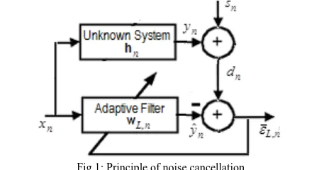
Conventional ANC employs two input signals to reduce the noise at the output of the system as illustrated in Fig 1. The primary input is the noise-corrupted signaldn. The reference inputxn, is measure of background noise alone which is in some way correlated with the noise in the primary. The output a priori errorL,n of this system at time
n is: n
n n
L, d yˆ
(1)
Fast Adaptive Filtering Algorithm for
Acoustic Noise Cancellation
M. Arezki, A.Namane, A. Benallal, P. Meyrueis and D. Berkani
[image:1.595.308.545.648.778.2]A
where yˆn wTL,n1xL,n is the model filter output,
T1 ,n n, ..., nL
L x x
x is a vector containing the last L
samples of the input signal xn, wL,n
w1,n, ...,wL,n
T is the coefficient vector of the adaptive filter and L is the filter length. The signal dn is the contaminated signal (Fig 2) containing both the clean speech sn and the noiseyn, assumed to be uncorrelated with each other. The primary input signal from the model is:n n n y s
d (2) n L n n y , T x h
(3)
where hn
h1,n, ...,hL,n
T represents the unknown system impulse response vector. The purpose of this system is to enable the system to control the filter until yˆn is as close to yn as possible.The error signal L,ncan be used to adapt the adaptive filter wL,n1 using some algorithm for filter adaptation. Several different algorithms for filter adaptation have been proposed. The filter is updated at each instant by feedback of the estimation error proportional to the adaptation gain, denoted asgL,n, and according to
n L n L n L n
L, w , 1 g , ,
w (4) The different algorithms are distinguished by the adaptation gain calculation.
III. PROPOSED SYSTEM A. Adaptive NLMS and FRLS Algorithms
The LMS Algorithms derived from the gradient [3], for which the optimization criterion corresponds to a minimization of the mean-square error. For the normalized LMS (NLMS) algorithm, the adaptation gain is given by:
n L n x n L c
L , 0 ,
, x g (5)
where is referred to as the adaptation step and c0 is a small positive constant used to avoid division by zero in absence of the input signal. The stability condition of this algorithm is 0<<2 and the fastest convergence is obtained for = 1 [12]. The power of input signal is estimated
byx,n (1)x,n1 xn2, where is a forgetting factor ( 1/L). The computational complexity of the NLMS algorithm is 2L multiplications per sample.
The RLS algorithm [3], for which minimizes a deterministic sum of squared errors. Fast versions of these algorithms are derived from the RLS by the introduction of forward and backward predictors. The FRLS algorithm shows a complexity of O(L). The adaptation gain is given by: FRLS , , RLS , 1 , , ~ n L n L n L n L n
L R x k
g
(6)T , , 1 , 1 T , ,
, Ln Ln Ln n i i L i L i n n
L x x R x x
R
(7)where RL,nis an estimate of the correlation matrix of the input signal vector and denotes the exponential forgetting factor (0 1). The variables L,n and ~kL,n respectively indicate the likelihood variable and normalized Kalman gain vector. Several numerical solutions of stabilization, with stationary signals, are proposed in the literature [7]. The computational complexity of the stabilized FRLS (NS-FRLS) algorithm is 8L per sample, and is stable, with the assumption of a white Gaussian input signal, under the following condition [7]:
L 2 / 1 1
(8)
B. Proposed Adaptive Algorithms
The numerical stabilization of the FRLS algorithm limits the range of the forgetting factor (8) and consequently their convergence speed and tracking ability. And the resulting of that algorithm has an 8L complexity.
In [11], they propose more complexity reduction. The modified and simplified FTF-type (M-SMFTF) algorithm [11], derived from the SMFTF algorithm [10], where the adaptation gain is obtained only from the forward prediction variables and using a recursive method to compute the likelihood variable. The computational complexity is 6L and its algorithm is stable, with assumption of a white Gaussian input signal, under the following condition [11]:
L
/ 1 1
(9) By a method of extrapolation [9], the autocorrelation matrix of order L is built starting from an estimate of the autocorrelation matrix of order P (P<<L). In this case, it is not anymore necessary to propagate prediction vectors of order L in the prediction part of the FRLS algorithm. If we denote P the order of the predictor and L the size of adaptive filter, the M-SMFTF algorithm can be easily used with reduced size prediction part. The computational complexity of the reduced size predictor M-SMFTF (RM-SMFTF) algorithm is(2L4P)2L and it is stable, with the assumption of a white Gaussian input signal, under the following condition [11]:
P
/ 1 1
[image:2.595.52.277.651.771.2] (10)
IV. SIMULATIONS
The noise reference input pass through the adaptive filter and output yˆn is produced as close a replica as possible of
n
y . The filter readjusts itself continuously to minimize the error between yn and yˆn during this process. The system output is:
n n n n
L, s y yˆ
(11)We can get the following equation of expectations:
2
2
, ) E( ˆ )
(
E Ln snynyn (12) Assuming thatxn and sn are not correlated and have zero means, we can write:
2
2 2
, ) E( ) E( ˆ )
(
E Ln sn ynyn (13) After convergence of the adaptive filter, explicitly,
n L,
w hn yˆn yn
L,n sn (14)A. Tracking Ability and Convergence
In the absence of the speech signal (sn=0). The expression (13) becomes:
2
2
, ) E( ˆ )
(
E Ln ynyn (15) The input signal xn used in our simulation is a white Gaussian noise, with mean zero and variance equal to 0.32. The impulse response of the system represents a real impulse response measured in a car and truncated to 256 samples. We compare the convergence speed and tracking capacity of the (NLMS, NS-FRLS, M-SMFTF and RM-SMFTF) algorithms. The filter length is L=256, the NLMS (=1) and NS-FRLS (11/3L) algorithms are tuned to obtain fastest convergence. The forgetting factor are respectively chosen for M-SMFTF and RM-SMFTF algorithms to 11/L and 11/P. The nonstationarity of the system to be modelled is simulated by
introducing a linear gain variation on the primary input signal. In Fig 3, we give the evolution, in decibels, of the mean square error MSE(n)(15). It shows that better performances in convergence speed are obtained for the proposed algorithm. It is observed that the proposed algorithm converges much faster and tracks better the variation of the system than both NS-FRLS and NLMS algorithms.
B. Noise Reduction
We define the input signal to noise ratio segmental [13], which is calculated on screens of a few milliseconds:
1 0 1 0 2 1 0 2 1 0 In 10log1 M k N i kN i N i kN i y s M
SNR (16)
where N is the size of the screen and M the number of screens. Same manner, we define the output signal to noise ratio segmental:
1 0 1 0 2 1 0 2 1 0 Ou t ˆ log 10 1 M k N i kN i kN i N i kN i s s s MSNR (17)
One of the qualifying criteria of the noise reduction algorithms is the increase measurement in signal to noise ratio. This criterion, noted GSNR and expressed in dB, is defined as the difference between SNRo u t and SNRIn for each screen, averaged on the whole of the screens:
In o u t SNR SNR SNR
G (18) We generate noisy speech signals with different SNRIn starting from files from clean speech signal alone and noise alone. We synthesize the noisy speech signals by adding the noise to the clean speech signal so as to reach the desired levels ofSNRIn. In our simulations, we took in the case of the NS-FRLS algorithm, 11/10L to ensure numerical stability.
The noisy speech signal with SNRIn= 30dB represents a case which we can say without noise (Fig 4). We observe (Fig 5a), that the output error of the system, which represents the estimated speech signal (L,n sˆn), is almost confused with the original speech signal except for the zones of silence (very weak power). We can say in these zones of silence, in absence of noise the NS-FRLS algorithm adapts less than the other algorithms. The curves (b) and (c) of Fig.5, which represent the temporal evolutions SNRo u t and
SNR
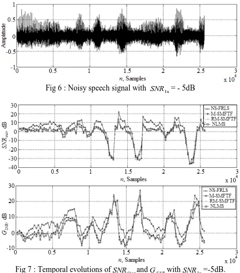
[image:3.595.42.284.571.739.2]G with SNRIn= 30dB, confirm well that the NS-FRLS algorithm adapts less than the other algorithms. In Fig 6, with SNRIn= - 5dB, we notice that the speech signal is relatively drowned in the noise. Fig 7 gives the temporal evolutions SNRo u tand GSNR. We can say that the NS-FRLS algorithm is slightly above the proposed algorithms.
Fig 3: Comparative performance of the algorithms,
L=256. M-SMFTF: =0.9961,=0.985, ca=0.5, E0=1;
RM-SMFTF: P=32, =0.9688, =0.9985, ca=0.5, E0=0.2;
Fig 8 represents the gain GSNR as a function of SNRIn. The original speech signal is combined with noise for
In
SNR between - 10dB and 20dB by steps of 5dB. We observe that, the gain GSNR decrease with SNRIn, the system has an overall tendency to not to remove the noise when SNRIn is strong and especially for the NS-FRLS algorithm. It is not necessarily a handicap; values beyond 15dB correspond relatively to slightly disturbed conditions, and attenuate the noise does not systematically improve comfort of listening. We notice that the NS-FRLS algorithm is placed slightly above the proposed algorithms.
V. CONCLUSION
From these performances criteria, measured by the mean square error MSE(n) and the gainGSNR, we have noticed that the proposed algorithms provide better results when making the noise less audible at exit of the system of noise cancellation. The simulations have shown that, the estimate of the noise have sensibly improved the adaptive performances in terms of noise reduction without distorting the speech signal. The NLMS algorithm is definitely less powerful than the other algorithms, and that the proposed algorithms allow a greater choice of compromise between these performances criteria and the computational complexity.
REFERENCES
[1] S. M. Kuo and D. R. Morgan, Active Noise Control Systems, New York: Wiley, 1996.
[2] M.Arezki, P.Meyrueis, N.Javahiraly, “Specific signal processing method for sound detected by an intrinsic optical fiber sensor”, Proc. SPIE 7675, 2010, 76750Q, Defense, Security, and Sensing, Orlando-USA, April 5-9, 2010.
[3] S. Haykin, Adaptive Filter Theory, 4th ed., NJ, Prentice-Hall, 2002. [4] L. Ljung, M. Morf and D. Falconner, “Fast calculation of gain
matrices for recursive estimation schemes,” Int. J. Control., vol. 27, 1978, pp.1-19.
[5] G. Caryannis, D. Manolakis and N. Kalouptsidis, “A fast sequential algorithm for least squares filtering and prediction,” IEEE Trans. Acoust. Speech Signal Process, vol. 31, 1983, pp.1394–1402. [6] J.CioffiandT. Kailath, “Fast RLS Transversal Filters for adaptive
filtering,” IEEE press. On ASSP, vol.32, no.2, 1984, pp.304-337 [7] M. Arezki, A. Benallal, P. Meyrueis, A. Guessoum and D. Berkani,
“Error Propagation Analysis of Fast Recursive Least Squares Algorithms,” Proc. 9th IASTED International Conference on Signal and Image Processing, Honolulu, Hawaii, USA, August 20–22, 2007, pp.97-101.
[image:4.595.308.554.56.335.2][8] G.V. Moustakides and S. Theodoridis, “Fast Newton transversal filters - A new class of adaptive estimation algorithms,” IEEE Trans. Signal Process, vol.39, no.10, 1991, pp.2184–2193.
Fig 4 : Noisy speech signal with SNRI n= 30dB
Fig 5 : Temporal evolutions: (a)MSE(n); (b)SNRO u t; (c)GS NR
L=256. M-SMFTF: =0.9961,=0.985, ca=0.5, E0=1;
RM-SMFTF: P=32, =0.9688, =0.9985, ca=0.5, E0=0.2;
NS-FRLS: =0.9996, E0=0.5; NLMS:=1.
Fig 8 : GS NRf
SNRI n
L=256. M-SMFTF: =0.9961,=0.985, ca=0.5, E0=1;
RM-SMFTF: P=32, =0.9688, =0.9985, ca=0.5, E0=0.2;
NS-FRLS: =0.9996, E0=0.5; NLMS:=1.
Fig 6 : Noisy speech signal with SNRI n= - 5dB
Fig 7 : Temporal evolutions ofSNRO u tandGS NRwithSNRI n=-5dB.
L=256. M-SMFTF: =0.9961,=0.985, ca=0.5, E0=1;
RM-SMFTF: P=32, =0.9688, =0.9985, ca=0.5, E0=0.2;
[image:4.595.47.298.390.763.2][9] P. P. Mavridis and G. V. Moustakides, “Simplified Newton-Type Adaptive Estimation Algorithms,” IEEE Trans. Signal Process, vol.44, no.8, 1996.
[10] A. Benallal and A. Benkrid, “A simplified FTF-type algorithm for adaptive filtering,” Signal processing, vol.87, no.5, 2007, pp.904-917.
[11] M.Arezki, A. Benallal, P. Meyrueis, and D. Berkani, “A New Algorithm with Low Complexity for Adaptive Filtering”, IAENG Journal, Engineering Letters, vol.18, Issue 3, 2010, pp.205-211. [12] D.T.M. Slock, “On the convergence behaviour of the LMS and the
NLMS algorithms,” IEEE Trans. Signal Processing, vol.42, 1993, pp.2811-2825.