Adaptive utility and trial aversion

www.elsevier.com/locate/jspi

Author’s Accepted Manuscript

Adaptive utility and trial aversion

B. Houlding, F.P.A. Coolen

PII:

S0378-3758(10)00373-3

DOI:

doi:10.1016/j.jspi.2010.07.023

Reference:

JSPI 4396

To appear in:

Journal of Statistical Planning

and Inference

Received date:

21 September 2008

Revised date:

3 July 2010

Accepted date:

26 July 2010

Cite this article as: B. Houlding and F.P.A. Coolen, Adaptive utility and trial aversion,

Journal of Statistical Planning and Inference

, doi:

10.1016/j.jspi.2010.07.023

Adaptive Utility and Trial Aversion

B. Houldinga,∗, F.P.A. Coolenb

a_{Discipline of Statistics, Trinity College, University of Dublin, Ireland.} b_{Department of Mathematical Sciences, Durham University, UK.}

Abstract

Decision making with adaptive utility provides a generalisation to classical Bayesian decision theory, allowing the creation of a normative theory for decision selection when preferences are initially uncertain. In this paper we address some of the foundational issues of adaptive utility as seen from the perspective of a Bayesian statistician. The implications that such a generalisation has upon the traditional utility concepts of value of information and risk aversion are also explored, with a new concept of trial aversion introduced that is similar to risk aversion, but which concerns a decision maker’s aversion to selecting decisions with high uncertainty over resulting utility.

Keywords: Bayesian Decision Theory, Uncertain Preferences, Risk, Expected Utility.

1. Introduction

The Bayesian paradigm coupled with the expected utility hypothesis of Bernoulli (1738) provides a transparent and compelling methodology for decision making in situations involving uncertainty. However, both in applications and on a theoretical level, it is traditionally assumed that the Decision Maker (DM) is able to state her correct utility value for any possible decision outcome, including those outcomes that have never been previously experienced. As such, classical Bayesian decision theory does not allow for a DM to learn or be surprised about her actual preferences.

The use of adaptive utility, as introduced by Cyert and DeGroot (1975), suggests a Bayesian model of preference learning, allowing for a Bayesian analysis of the decision problem even when the DM is unable to fully specify her true preferences. In this setting the DM is permitted to be uncertain over her true preferences, with the appropriate utility function only being known up to the value of an uncertain parameter

θ. Such a parameter can be used to model uncertainty over any aspect of the DM’s preferences, with interesting examples including vectors of unknown trade-off weights or unknown level of risk aversion. The DM’s beliefs over such a utility parameter are stated, with learning taking place via Bayesian updating once the DM receives extra information concerning her true preferences. The information concerning the DM’s preferences can then take many forms,e.g., the suggestion by Cyert and DeGroot whereby the DM notes the sign of the difference between the prior expected value of the utility outcome (with respect to beliefs over the uncertain utility parameter) and the actual utility value that is received.

Whilst it is noted that there are already several works in various disciplines that consider the problem of decision making with unknown preference, there appears not to be any formal analysis of this situation from the perspective of the Bayesian decision theorist. Moreover, there appears not to be any consideration of the implications of uncertain preferences for traditional decision theory concepts such as value of information or risk aversion. This work seeks to address these issues.

The format for the remainder of this paper is as follows. Section 2 introduces an adaptive utility function, discusses motivation for its use, and provides a review of similar theories. Section 3 discusses foundations and the interpretation of a utility parameter. Section 4 considers the implications for value of information and Section 5 considers the implications for risk aversion. Section 5 also introduces a new concept of trial aversion that only exists when a DM has preference uncertainty. Finally, Section 6 concludes with a discussion of potential directions for future research.

2. Adaptive Utility and Uncertain Preferences

To introduce the type of decision problem considered here, imagine a DM who is faced with a decision problem in which there are at least two possible courses of action, and denote byRthe set of all possible outcomes that may result from decision implementation. Once Rhas been identified, then each available decisiondcan be associated with a probability distributionPr|dwhich quantifies the DM’s belief in obtaining

outcomer∈ Rif decisiondis indeed implemented.

In such a setting we would like to generate a utility function that takes as its input the set of available decisions, and which returns a real number used for representing the DM’s preference for that decision. This will then enable the creation of a complete binary preference rankingthat is used to determine preference between any two available decisions. That is to saydidj denotes that decisiondi is at least as preferable

as decisiondj. In practice, however, the identification of such a utility function that has domain the set of

available decisions will not be straightforward. Instead it may be more appropriate for the DM to identify a utility function that has domain the set of possible decision outcomesR, and then to use this to reconstruct the utility values for the set of available decisions.

In order to relate a utility function that has domain the set of decision outcomes to one which has domain the set of available decisions, the concepts of a ‘mixed’ decision and a ‘degenerate’ decision are introduced. A degenerate decision is one that leads to a particular outcome with certainty, and we can associate a degenerate decision with every element ofR. A mixed decision is one in which there exists uncertainty as to its outcome, and as such, can be considered as a probability distribution over the set of degenerate decisions. Here we employ a common notational convention wherebyp1d1+· · ·+pndn, withpi≥0 and

n

i=1p1= 1,

denotes the mixed decision that results in outcomerj with probability

n

i=1piPr|di(rj). The union of the

collection of degenerate decisions and mixed decisions then results in a convex set D, with the degenerate decisions forming the convex nodes.

The expected utility hypothesis of Bernoulli (1738) argues that a DM should make decisions by seeking to maximise the expected utility of the outcome. This hypothesis was later proved by von Neumann and Morgenstern (1947) under the assumption that the DM agrees with a small collection of axioms of rational choice. Additional axiomatic developments for when probabilities are subjective (e.g., Anscombe and Aumann (1963), or Savage (1954)), or for if there are an infinite number of possible outcomes (e.g., Herstein and Milnor (1953)), were later developed.

Under the setting of the above, the main result of von Neumann and Morgenstern is that, if a DM agrees with a small number of axioms of rational choice, then there exists a unique function u(up to a positive linear transformation), with domain the set of decisionsD and co-domainR, satisfying properties P1 and P2 below:

P1: For alldi, dj∈ D, u(di)≥u(dj)⇔didj.

P2: For alldi, dj∈ Dand any α∈(0,1),u(αdi+ (1−α)dj) =αu(di) + (1−α)u(dj).

The second property implies that utilities have a cardinal meaning, and do not simply rank decisions. It also explains how utilities for non-degenerate decisions can be formed from utilities for degenerate decisions, hence giving rise to the expected utility representation for when mixed decisions are considered (in what follows we will discuss utility as a function with domainDorRinterchangeably, but on the understanding that the utility of a mixed decision is found through implementation of property P2).

Nevertheless, the result of von Neumann and Morgenstern only states that there exists a unique function satisfying both properties P1 and P2. Hence, there is still the problem of identification before this function can be employed within a decision analysis. To determine the utility value of a particular decision outcome

r, the DM can use the system described by DeGroot (1970) of comparing the gamble that returnsr with certainty to a gamble that returns the best possible outcome with probability p, or otherwise returns the worst possible outcome. If the DM’s utility function is scaled to cover the interval [0,1], then the value ofp

making the DM indifferent between either gamble will be equal tou(r).

This elicitation system bounds the utility function to the interval [0,1], but as a utility function is only unique up to a positive linear transformation, the interval can be extended to any arbitrary finite interval [a, b]. The restriction to a finite interval is natural if we do not wish to allow the possibility of one outcome being deemed infinitely better (worse) than another outcome, meaning that the DM would always select (reject) any decision that had positive probability of resulting in that outcome, regardless of how small that probability would be. This is often referred to as the ‘no heaven or hell’ assumption, and is included in the von Neumann and Morgenstern theory through their Archimedean axiom; indeed, it was the St. Petersburg paradox of infinite expected return that led to the expected utility hypothesis of Bernoulli.

Nevertheless, in practice, and for the purposes of application, it is common to assume the appropriate utility function follows a general form with particular properties,e.g., the logarithmic function suggested by Bernoulli for monetary returns. However, neither the construction approach, nor the method of assuming a particular form, considers the possibility that the DM may be uncertain of her actual true preferences. Yet in reality it is perfectly natural for a DM to be unsure of her preferences. A DM could, for example, be considering an outcome that would not be received until some future time point, and then she will need to consider how her preferences may have evolved by the time of outcome realisation.

Additional scenarios include situations where outcomes are multi-attributed,e.g., Keeney and Raiffa (1976). In such settings a DM may be fully able to identify marginal utilities for specific attribute levels, but still be uncertain about the way the attribute levels interact when forming an overall utility. For the purpose of illustration, we could imagine a DM who needs to make a journey and has the choice of various methods of transportation, all of which having differing cost levels and transport time. A DM may be able to identify a marginal utility for the cost of making a journey, or a marginal utility for journey duration. However, it may be that the overall utility is not simply the unweighted sum of such marginal utilities, but that the preference for a specific cost level is impacted by the actual journey duration, or that cost implications are more important than travel duration. In such a situation, utility uncertainty may arise through uncertainty in the level or nature of the interaction and/or combination of the marginal utilities.

Parametric utility models are also subject to utility uncertainty if it is agreed that such models should follow a general family form, but where a parameter indicating aspects such as shape or curvature (e.g., determining level of risk aversion) is assumed unknown. In general though, the theory of decision making under uncertain preferences would appear most useful for when a DM is facing a decision problem in which there is the opportunity of experiencing novel or unfamiliar outcomes. As Simon (1955) states, “the [DM] ... does not know how well [she] likes cheese until [she] has eaten cheese”. Rather than assuming that the DM’s strength of preference and corresponding utility for every outcome is known, the theory of adaptive utility permits a DM to be uncertain, and to instead learn about her preferences.

sug-gested a model whereby the DM’s utility for a decision not only depended on the eventual outcomer, but also on an uncertain parameterθ. Such a parameter is included within notation as a conditioning argument,

e.g.,u(r|θ) oru(d|θ), and it is envisioned that the DM will learn about its value through information that is observed following decision selection. When expressed in this way Cyert and DeGroot refer to the function

uas an adaptive utility function, however, for the purpose of this work we suggest that an adaptive utility function be defined to be au(r) =Eθ[u(r|θ)] andau(d) =Eθ[u(d|θ)], i.e., the expected value of Cyert and

DeGroot’s function with respect to beliefs over the parameterθ. The functionu(·|θ) will instead be referred to as a classical utility function.

If only a single decision is required the strategy of seeking to maximise expected adaptive utility is no different to classical utility theory under the assumption that true preferences are equal to current expected preferences. However, in a sequential decision problem the DM can find it beneficial to initially select decisions that appear sub-optimal under current expected preferences. This is because information gained following selection of the first decision may depend on the decision that was selected, and so it can be beneficial to initially select decisions which are more likely to be informative ofθ. This situation provided motivation for Houlding and Coolen (2007), where the use of adaptive utility theory within sequential decision problems relating to system failure correction was illustrated, and where a general solution algorithm for ann-period problem was given.

Additional works that seek to incorporate uncertain preference within a decision making paradigm include Crawford and Shum (2005) (the problem of drug selection faced by Italian doctors) and Erdem and Keane (1996) (liquid detergent brand selection by US customers). Both consider decision making with uncertain preferences in order to model data on actual decision selection, with preference uncertainty claimed to arise through uncertainty over the attribute levels of the resulting decision outcome, e.g., symptomatic and curative efficacy of anti-ulcer drugs. The theory of adaptive utility can also cater for the situation in which the utility of a decision is uncertain due to uncertainty over the attribute levels of possible outcomes. However, this is not necessary and adaptive utility will still permit uncertain preferences even when the attribute levels of all possible outcomes are known.

Chajewskaet al.(2000) consider an adaptive approach to utility elicitation for the problem a decision analyst faces when seeking to determine the utility function of another individual. The analyst is seeking to identify the appropriate decision choice for their client, and is able to elicit their client’s utility for various options by asking a series of questions. The main result of Chajewskaet al. is the development of an algorithm for doing this optimally, i.e., for asking the minimum number of questions necessary in order to identify the correct decision. The main difference between the approach of Chajewskaet al. and the approach described here is that, rather than seeking to elicit another person’s preferences, we refer to a situation of uncertainty in personal preference.

Uncertain preferences also arise in the work of Cohen and Axelrod (1984), where uncertainty exists over whether or not a decision making model has been miss-specified (this theory was applied in a model for optimal marketing by Fraser and Hite (1988)). The important difference between the theory of adaptive utility considered in this paper and the theory of Cohen and Axelrod is that here true preferences, though unknown, are not assumed to change. Cohen and Axelrod instead consider a situation in which decision making experiences actually alter the DM’s underlying utility.

Another approach is taken by Ben-Haim et al. (2009), where an Info-gap model is assumed for utility uncertainties in cholesterol management. Rather than incorporating an uncertain parameter representing utility uncertainty, Ben-Haim et al. consider a situation where uncertainty is so severe that, other than the specification of a best point-estimate guess, nothing else can be specified. In particular, there is no probabilistic specification of how accurate such a best point-estimate guess may be. Instead a nested subset of possible horizons of uncertainty is specified and the decision selected which is deemed most robust in that it guarantees a specified minimum critical return for the largest horizon of uncertainty. Unlike the imprecise theory of Farrow and Goldstein, or the parametric theory discussed here, the Info-gap approach of Ben-Haim et al. is non-probabilistic, and can not quantify, or even given bounds on, the probability of outcome for any quantity that is subject to ‘info-gapping’.

In general, the theory of adaptive utility presented here forms part of the wider topic of Bayesian Robustness, but where the DM seeks to be robust with respect to the utility function, see e.g., Berger (1993) and R´ıos Ins´ua and Ruggeri (2000) for further information on Bayesian Robustness. The result of a Bayesian statistical analysis will be dependent on the form of the model proposed and the specification of certain model parameters. In many situations, however, allowing model parameters (or even the model itself) to change slightly does not influence greatly the conclusions that can be drawn from the inference, and only when results are highly dependent on specific parametric values would there be concern on the appropriate value for a parameter. The adaptive utility model presented here allows a DM to remain uncommitted to a specific utility parameter, hence allowing investigation as to the effect that certain utility parameter values or prior distributions will have on the resulting optimal decision strategy.

Finally, both Arrow (1995) and Dekelet al.(2001) consider utility uncertainty through a model of unforeseen contingencies. Arrow considers this setting in a philosophical discussion of how freedom can be represented through flexibility, proposing the same function as the adaptive utility function considered here as a method of ordering decisions according to their flexibility. Dekel et al., however, do not consider a probabilistic representation of possible utility functions, instead providing a formal expected utility representation ofex ante preference given a set of possibleex post preferences known as the subjective state space.

Whilst both this work and that by Arrow are concerned with the same function for representing preference, our motivation is based on examining implications for Bayesian statistical decision theory, rather than discussing the philosophical meanings of freedom. This paper also differs from Dekel et al. in that we are concerned with a probabilistic description of preference, though we appreciate that this is achieved by presuming that a prior subjective distribution over the utility parameter is available before the problem is analysed. Although this is clearly weaker than the desired aim of developing a theory in which the DM’s subjective beliefs over possible utility functions can be determined from herex antepreference, we note that for the purposes of application, and also for examination of the implications for value of information or risk aversion, this is not necessary.

3. A Parameter for Preference

As mentioned in Section 2, we define an adaptive utility function as _au(r) = Eθ[u(r|θ)], so its value

for any particular decision outcome rwill depend on the DM’s beliefs over the utility parameter θ. Cyert and DeGroot (1975) introduced such a utility parameter in order to encapsulate the uncertainty a DM has about her preferences. However, the main aim of Cyert and DeGroot appears to be the introduction of the uncertain utility concept and in discussing implications for economic theory. As such, neither the interpretation of the utility parameter, nor its role within the foundations of decision theory, are considered. Furthermore, in order to make the assertion that a DM should select decisions in order to maximise the expected adaptive utility of the outcome, an argument detailing the normative validity of this strategy should be given.

from that which is commonly referred to as the state of nature. Whilst the state of nature determines the actual outcome following decision selection, the state of mind determines the actual utility for that outcome. Property P1 of a utility function states that such a function will uniquely (up to a positive linear transformation) be in agreement with a given complete binary preference orderingover the set of decisions

D. Hence, other than changes in the value ofθthat are equivalent to taking a positive linear transformation of u(·|θ), each change of θ will be equivalent to a change in the preference ordering . That is to say, a state of mind fundamentally represents a possible preference rankingθ overD, and as such, the adaptive

utility setting discussed here assumes that a true preference relation overDexists, but that the DM may be uncertain about it.

Hence a state of mindθis a well-defined random quantity in the de Finetti (1974) sense, and so a probability distributionPθ may be specified over its value. This random quantity can be observable or unobservable.

An important example of an observableθwould be the situation where it represents the DM’s utility value (on a given scale) for some novel decision outcome. If the utility of such an outcome is uncertain, then the DM may ‘observe’ θ by experiencing the unfamiliar outcome and noting whether or not she found it preferable to alternative known outcomes. In other situationsθmay be unobservable, and this would be the case if following decision implementation the DM experienced a feeling of either elation or disappointment in comparison to what had been anticipated under Pθ. In this case elation would mean thatPθ had been

too pessimistic, but not necessarily indicating by how much, whilst disappointment would mean thatPθhad

been too optimistic, but again, not necessarily indicating by how much.

As preferences are inherently subjective, it is natural to assume that distribution Pθ is also subjective.

However, the use of a subjective distribution for representing beliefs overθ leads to further issues in the distribution’s elicitation and interpretation, both of which are traditionally based on the use of scoring rules (see again de Finetti (1974)). For this reason we assume that such a scoring rule is known (or at least one is assumed), for otherwise we would regressad infinitum. In essence then, the use of adaptive utility in decision selection is analogous to the use of a hierarchical prior in Bayesian analysis (see,e.g., Berger (1993)). As discussed above, a utility value corresponds to a probability value. When scaled to fall in the interval [0,1], the utility of any decision outcome r is interpreted as the probability value pmaking the DM indifferent between obtaining r for sure, or playing the gamble paying best possible outcome with probability pand worst possible outcome otherwise. Adaptive utility theory simply permits the DM to be uncertain aboutp, with the DM instead specifying a probability distribution over its value.

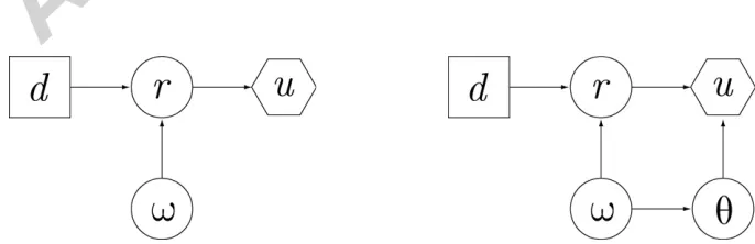
Beliefs overθmay depend on beliefs over the true state of nature, to be denoted byω, but unlike the state of nature, the value ofθdoes not affect actual decision outcome. In order to demonstrate the role that the state of mind plays in the decision problem, Figure 1 gives influence diagrams for the classical situation and the adaptive utility situation (see Shachter (1988) and the references therein for details on the construction and interpretation of influence diagrams). Note that in the adaptive utility case the influence diagram explicitly permits probabilistic dependence between the state of mind and state of nature. Independence would be represented by deleting the arrow connecting theωandθ nodes.

As an example of a situation where it would be reasonable to accept probabilistic dependence between the state of mind and state of nature, consider the following: on each day a kiosk sells either ice-creams or hot dogs, with the item on sale, represented by the state of natureω, being decided by a manager at the beginning of the day depending on what he believes will be the weather for that day. A DM’s preference between consuming an ice-cream or a hot dog, as characterised by her state of mindθ, is also assumed to depend on the weather. In this situation it would be reasonable to accept that beliefs over ω and θ are dependent, but conditionally independent given knowledge of the weather.

The use of a state of mind within adaptive utility decision making is thus closely related to the concept of state-dependent utility (examples of works considering state-dependent utility can be found in, for example, Karni (1993) or Schervishet al. (1990)). State-dependent utility alters a DM’s preferences depending on the state of nature that occurs, and is usually removed in classical utility theories which consider only state-independent utility (e.g., Anscombe and Aumann (1963)). State-dependency, however, is similar to the adaptive utility concept where the DM’s preferences may change depending on the true state of mindθ. The difference being that the state of mind, unlike the state of nature, does not affect the actual outcome of decision selection.

Given a distributionPθrepresenting beliefs over a state of mind, we demonstrate that the DM should select

decisions so as to maximise adaptive utility (rather than any other functional of Pθ) by making repeated

use of the uniqueness and existence of a traditional utility function. In doing so we claim that the adaptive utility function au(·) =Eθ[u(·|θ)] exists and is the unique function (up to positive linear transformation)

satisfying the following two properties:

P3: For alldi, dj∈ D, au(di)≥au(dj)⇔didj.

P4: For alldi, dj∈ Dand any α∈(0,1),au(αdi+ (1−α)dj) =αau(di) + (1−α)au(dj).

The above is of course a generalisation of the main result of von Neumann and Morgenstern (1947), returning to that result whenPθis a degenerate distribution. In effect this means that the adaptive utility function is

the DM’s actual utility function for this setting. That is not to say the adaptive utility function represents the true underlying preferences of the DM, and only whenPθ is degenerate can this be certain. Rather, the

adaptive utility function is representing the DM’s preferences over decisions when it is accepted that true preferences are uncertain and when such uncertainty is modelled by distribution Pθ. In other words, the

adaptive utility function represents preferences over decisions prior to any further information concerning preferences over possible decision outcomes.

The argument behind the existence of the function _au(·) is clear following the existence of each possible classical utility function u(·|θ) and because_au(·) is well-defined for a given distributionPθ. Furthermore,

property P4 is easily verified as a result of each possible classical utility satisfying corresponding property P2 and because expectation is a linear operator. Hence, all that remains to be shown is that the adaptive utility function is the unique function in this setting that satisfies property P3.

To proceed we consider a decision outcome set aR consisting of all possible classical utility values for all

possible decisions. This means that, in addition to a decision being associated with a distribution overR, it will also be associated with a distribution overaR. Repeated application of von Neumann and Morgenstern’s

result means that there exists a unique (up to a positive linear transformation) utility functionu∗:aR →R

representing preferences over elements ofaR. Presuming the set of possible classical utility functions have

been scaled to ensure they are commensurable, such a utility function can simply return the original value that was the element of aR. Property P2 of a classical utility function can then be used to extend the

To ensure commensurability of elements of aR, i.e., to ensure it is meaningful to compare utility values

that are conditioned under differing values of θ, each possible utility function u(·|θ) must be placed on a suitable scaling. As Boutilier (2003) notes, the strategy of selecting decision so as to maximise expected adaptive utility is not invariant to the scaling of the original possible utility functions. To illustrate this problem consider the two possible utility functions u(di|θ1) = 2iand u(di|θ2) =I{i=1} for i∈ {1,2} (here

I{i=1} is the usual indicator function returning 1 ifi = 1 and 0 otherwise). If prior beliefs are such that

Pθ(θ1) =Pθ(θ2) = 0.5, then the adaptive utility maximiser should select decisiond2. However, the function

˜

u(di|θ2) = 3I{i=1} is a positive linear transformation of u(di|θ2), and thus represents exactly the same

preference relation between decisionsd1 and d2. Yet when ˜u(·|θ2) is used, the adaptive utility maximiser

should select decisiond1. Hence the issue is, knowing thatu(·|θ2) and ˜u(·|θ2) (along with the infinite number

of alternative positive linear transformations) represent exactly the same preference ordering over decisions, which one is appropriate for use within expected adaptive utility calculations?

Boutilier resolved this problem by making an assumption of extremum equivalence. This assumption requires that, under each possible utility function, there exists the same most favourable outcome and the same least favourable outcome. Furthermore, each possible utility function is assumed to give the same utility for the best outcome and the same utility for the worst outcome. When extremum equivalence does hold, Boutilier shows that by viewing the decision problem as the selection of a compound gamble in which the first stage is a gamble over the utility function and the second a standard gamble over decision outcome, then there exists a method of scaling possible utility functions to ensure commensurability.

Extremum equivalence, however, is an unreasonable assumption in many decision problems. For example, we may wish for a particular state of mind to represent a preference reversal, or for the strength of preference between the best outcome and the worst outcome to vary. In order to find a system of scaling possible utility functions so as to make them commensurable without requiring extremum equivalence, we can consider a decision outcome as a pair listing the actual outcome r and the state of mind θ. When viewed in this way, the utility value of an outcome can be determined through the usual construction approach of finding probability values that lead to indifference between certain gambles. Assuming that (r∗, θ∗) is the best outcome and state of mind pair (i.e., receivingr∗ ifθ∗is true is at least as preferable to receiving any other outcome under any other state of mind), and that (r∗, θ∗) is the worst outcome and state of mind pair, the utility value of any other outcome and state of mind pair (r, θ) is equal to the value p∈[0,1] such that the DM is indifferent between receiving (r, θ) for certain, or playing the gamble leading to (r∗, θ∗) with probabilitypand (r∗, θ∗) otherwise.

This construction method requires the DM to consider her preferences over outcome and state of mind pairs, which will of course be a very difficult elicitation problem and a far from trivial task in all but the simplest of scenarios. It requires the DM to make hypothetical choices that are not actually available, for only one value ofθwill be correct. Moreover, if the possible values forrandθare intervals in R, then it requires the DM to specify an ordering overR2, for which there is no natural method. Indeed, it would appear to be the main weakness of preventing the framework from being applied formally.

It is also of note that failure to be able to determine preferences over pairs such as (r, θ) and (r, θ) could be resolved by regressing to an additional uncertain parameter φ that determines these, but as with the previous analogy to hierarchical priors, it is hoped that only one additional level of hierarchy is sufficient to allow a Bayesian model for preference learning.

The above construction method bounds all adaptive utility values to the interval [0,1], and a suitable positive linear transformation can then be used to change this to any finite interval [a, b]. However, if the DM already has known possible utility functions u(r|θ1), u(r|θ2), . . ., then the process of scaling them to

ensure commensurability becomes a little simpler. To do this, first specifyu(r∗|θ∗) = 1 andu(r∗|θ∗) = 0 (which implicitly rejects the trivial situation where all situations are considered equally desirable). Using notation such that (p1a1, . . . , pnan) represents a distribution where outcome ai occurs with probabilitypi,

each classical utility function is scaled in the following way:

1. Ifu(r|θk) is such thatu(rs|θk) =u(rt|θk) for allrs, rt∈ R, thenu(r|θk) =p, withp∈[0,1] such that

the DM is indifferent between (r, θk) for sure and the gamble

p(r∗, θ∗),(1−p)(r∗, θ∗).

2. Otherwise there existsrθk, rθk∈ Rsuch that, for any other r∈ R, we have the relations:

• u(rθk|θk)≥u(r|θk)≥u(rθk|θk)

• u(rθk|θk)> u(rθk|θk).

Such a utility function is then scaled using the two constraints:

• u(rθk|θk) =qθk

• u(rθk|θk) =qθk

whereqθk, qθk∈[0,1] are the values selected which make the DM indifferent between (rθk, θk) for sure and the gambleqθk(r∗, θ∗),(1−qθk)(r∗, θ∗)

, and similarly between (rθk, θk) for sure and the gamble

q_θ

k(r

∗_{, θ}∗_),(1−q

θk)(r∗, θ∗)

.

4. Value of Sample Information

Even though several authors have considered decision problems when preferences are uncertain, there appears to have been no discussion on the effect that utility uncertainty has upon classical diagnostics such as value of information or risk aversion. The concept of value of sample information, that arises as a diagnostic in the type of decision problem considered here, is discussed by DeGroot (1984). Further discussion can also be found in, for example, Bernardo (1979), DeGroot (1962), and Raiffa and Schlaifer (1961).

Let observable random quantity X represent a currently unknown piece of information. In discussing the expected amount of information inX, or the expected value ofX, we are referring to its fair utility value,

i.e., the maximum amount of utility the DM would forgo in order to know X. In a decision problem, the expected value ofX is the expected difference between the maximum expected utility obtainable through decision selection with knowledge of X, and the maximum expected utility obtainable without knowledge ofX. Alternative meanings are not considered here, but can be found in Goel and Ginebra (2003).

The set of possible valuesX can take will be denoted byX, and a particular value byx. Under this notation, problems of interest in the classical treatment of value of sample information occur whenX can inform the DM about the likely outcome of an available decision,i.e., if there exists a possible combination of outcome

Iω(x), and the value of unknown informationX byIω(X) (with subscriptω representing the true state of

nature,i.e., that determining the decision outcome following decision selection). AsX is a random quantity, then so isIω(X), and its expected value,EX[Iω(X)], is defined by:

EX[Iω(X)] =EX

max

d∈D{Eω|X[u(d)]}

−max

d∈D{Eω[u(d)]} (1)

In a classical known utility setting, the Expected Value of Sample Information (EVSI) depends only on the following components of the decision problem: the set of feasible decisions withinD, the utility functionu, the distributionPωrepresenting prior uncertainty over the state of nature, and the likelihood functionPX|ω.

The introduction of uncertain preferences, however, leads to interesting questions regarding the classical treatment of value of information. The above equation for the EVSI must be generalised for use with adaptive utility, and it is of interest to consider what effect utility uncertainty will have. Furthermore, it is now possible to learn about preferences following appropriate decision selection, and we may wish to quantify the value of such state of mind specific information.

In approaching such problems we first consider the situation in which beliefs over the state of nature, ω, and the state of mind,θ, are independent, and we begin by considering the case that informationX is only relevant for learning aboutω. Under these assumptions we argue that the EVSI should be measured by the following (where notationIωis replaced byaIωto highlight that we are now considering an adaptive utility

setting):

EX[aIω(X)] =EX

max

d∈D{Eω|X[au(d)]}

−max

d∈D{Eω[au(d)]} (2)

Equation (2) is clearly a generalisation of Equation (1), with the only difference being that the adaptive utility function _au(d) replaces the known utility function u(d). Indeed, Equation (2) returns to Equation (1) in the case thatPθ is degenerate. However, the important difference is that now, in addition to those

components of the decision problem listed above, the DM’s beliefs over her state of mind, as represented by

Pθ, affects the EVSI concerningω.

As an example of how beliefs over θ can affect the EVSI, consider the decision problem with available decisionsdA anddB subject to the following pay-off matrix:

ω1 ω2

dA r1 r2

dB r2 r1

Prior beliefs are such thatP(ω1) =P(ω2) = 0.5, and the DM’s likelihood function is such that information

X will fully inform the DM of ω, i.e., PX|ω(xj|ωi) = δij for j = 1,2 (with δij representing the usual

Kronecker delta). Thus the predictive distribution is P(x1) = P(x2) = 0.5. Beliefs over preferences are

assumed to be such thatP(θ1) =p= 1−P(θ2), withp∈[0,1]. Commensurable utilities are assumed to be

u(r1|θ1) =u(r2|θ2) = 1 andu(r2|θ1) =u(r1|θ2) = 0. Note that the commensurability assumption included

here implies that, out of the two possible decision outcomesr1andr2, the utility for obtaining the preferred

outcome is the same regardless of whether this isr1 orr2. Similarly, there is no additional loss in obtaining

the dis-preferred outcome regardless of whether it was discovered to ber1or r2.

as a function ofp. Assuming thatθ1 = 1 andθ2 = 0, Figure 2 plotsEX[aIω(X)] andV[θ] over the range

p∈[0,1], demonstrating thatEX[aIω(X)] monotonically decreases asV[θ] increases.

Figure 2: EX[aIω(X)] (solid) andV[θ] (dashed) forp∈[0,1]

The results of this example suggest the hypothesis that a decrease in uncertainty overθ necessarily leads to an increase in EVSI for information relevant in determining the state of nature. A reason for this could be that, if the DM is uncertain about her preferences, then she will be unsure over which decision outcome she should aim for, and thus information concerning the likely decision outcome following selection of any specific decision is of little use. Nevertheless, although this is the case in the given example, it is not generally true that the expected value of such information will only increase as uncertainty concerning preferences decreases.

Before providing a counter example, we note that uncertainty can be measured in a number of different ways. For example, Gould (1974) considers measuring uncertainty by variance, the Shannon and Weaver (1949) measure of entropy, and the Rothschild and Stiglitz (1970) measure of spread in distributions with equal mean (under whichY1 is deemed more uncertain thanY2 ifY1=Y2+, where, conditional uponY2,

is uncorrelated random noise with mean 0 and positive variance). Gould demonstrates that in the known utility situation with finite state of nature space Ω, EVSI does not necessarily increase when the number of elements in Ω having non-zero probability increases, less probability is concentrated on any single element of Ω, the variance ofω increases, or uncertainty overω in the Rothschild and Stiglitz sense increases.

To provide a counter example to the hypothesis that EVSI only increases as uncertainty concerning prefer-ences decreases, consider again the previous problem, but where now commensurable utilities are such that

u(r1|θ1) = u(r2|θ1) = 1, u(r1|θ2) = 0, andu(r2|θ2) = 2. As an aside, note that here commensurability

implies that if θ2 were true, then there is a definite preference for r2 over r1, whilst under θ1, the DM is

indifferent betweenr1 andr2. Moreover, if indifference did not exist then there is increased utility gain if

the DM selects the preferred outcome, and reduced utility if the DM selects the undesired outcome. As an example, one could consider two unfamiliar fruitsfAandfB. IffAwas just as nice asfB then their utilities

would be equal. If, however,fB was nicer thanfA, then the DM may derive additional utility in having

selected the better fruit than they would have done in the case of indifference,e.g., a utility for having made the correct choice. Similarly, there may be a loss of utility in having selected the less nice fruit, even reduced from that which would have been derived from obtaining the same fruit but in a situation of indifference,

e.g., a utility for having made the wrong choice. Alternatively, this setting could model a situation where, underθ1, the DM is indifferent between fruits, whilst under θ2, the DM enjoys certain types of fruit such as

r2, but actively dislikes other types of fruit, such asr1, because they may be sour and bitter.

In this caseEX[aIω(X)] monotonically increases aspdecreases. Assigningθ1 = 1 andθ2= 0 again allows

necessarily decrease as more elements of Θ have non-zero probability, neither does it necessarily decrease as greater probability is assigned to any single element of Θ. Furthermore, the EVSI is not necessarily minimal when elements of Θ are equally probable.

Figure 3: EX[aIω(X)] (solid) andV[θ] (dashed) forp∈[0,1]

A further result is that the EVSI does not necessarily increase asV[θ] is decreased, and this result is invariant to the numerical representation assigned toθ1 and θ2. This is because the numerical assignment will only

affect the value ofV[θ], and not the EVSI. Assigning a generic representation ofθ1=v1 andθ2=v2, with

v1, v2 ∈R and v1 =v2, V[θ] is given as p(1−p)(v1−v2)2. Hence, as a function of p, V[θ] is maximised

whenp= 0.5 and monotonically decreases aspmoves away from this value. In the example, however, the EVSI is monotonically increasing inpand so both the EVSI andV[θ] will decrease aspincreases from 0.5 to 1, regardless of the values assigned forθ1 andθ2.

In the known utility setting, Gould (1974) argued that no simple relation exists between EVSI and uncer-tainty overωbecause, all other factors being equal, a change in uncertainty overωaffects both the maximum expected utility consideringX,EX

maxd∈D{Eω|X[u(d)]}

, and the maximum expected utility not consid-eringX, maxd∈D{Eω[u(d)]}, the difference of which forms the EVSI. This argument also explains why an

increase in uncertainty overθdoes not necessarily lead to a decrease in EVSI. A change in beliefs overθcan affect both the value of the maximum expected adaptive utility consideringX,EX

maxd∈D{Eω|X[au(d)]}

, and the maximum expected adaptive utility not consideringX, maxd∈D{Eω[au(d)]}, the difference of which

gives the EVSI when preferences are uncertain.

An increase in uncertainty over θ can only lead to a decrease in EVSI if EX

max_d∈D{Eω|X[au(d)]}

is decreased (increased) by more (less) than max_d∈D{Eω[au(d)]}. In both the first example and the counter

example, max_d∈D{Eω[au(d)]} does not depend on the value of p. However, whilst in the first example

EX

max_d∈D{Eω|X[au(d)]}

Information X need not only be informative of the state of nature, with an alternative being that X is a vector of independent values (X1, X2), with X1 being informative ofω only and X2 being informative of

the state of mind only. As the state of mind is a parameter influencing subjective preference, the type of information relating to its value is likely to be quite different from the type of information used in updating beliefs concerning actual decision outcome. However, possibilities include the actual experience of a novel outcome, or perhaps experiencing an alternative outcome that is believed to have utility which is correlated or exchangeable with that of the novel outcome, e.g., tasting the unfamiliar cheese, or experiencing some other dairy product. Introspection, conversation with friends who are believed to share similar preferences and are more experienced, the viewing of advertisements, or advice from impartial (or possibly biased) experts are all also possible so long as a subjective likelihoodPX|θcan be expressed.

In this situation the EVSI is expressed by the following (where notation is such that if X is relevant toθ, then it is included as a conditioning argument in the adaptive utility function):

EX[aIω,θ(X)] =EX

max

d∈D{Eω|X1[au(d|X2)]}

−max

d∈D{Eω[au(d)]} (3)

As discussed in Houlding and Coolen (2007), interesting problems in adaptive utility theory are necessarily of a sequential nature, where information about the state of mind is received following appropriate decision selection. Just as is the case of traditional EVSI, it can be shown that the EVSI of information relating to the state of mind can only decrease if it is to be received later in the sequential problem. As a consequence of this, if there exists a decision that, although not appearing optimal under current beliefs about preferences, is the only decision that offers opportunity to learn about the true state of mind, then either the DM should select that decision immediately in the sequential problem, or not at all.

To determine the EVSI within an n-period sequential problem we assume that in periodi the DM selects decisiondi _{and observes decision outcomer}i _{that is used to update her beliefs over the state of nature. We}

also assume that following selection of di _{the DM observes utility information z}i_{, independent ofr}i_{, that}

is used to update her beliefs over the state of mind, e.g., she discovers a new utility value, or experiences a utility that may be correlated or exchangeable with another that is unknown, or she records elation or disappointment from that which she had anticipated.

Hence the decision making history immediately before selection of decisiondi _{can be represented by vector}

Hi= [(d1, r1, z1), . . . ,(di−1, ri−1, zi−1)]. In this setting the DM’s beliefs over the state of nature and her state of mind immediately before selection ofdi will be represented by posterior distributionsPω|Hi and Pθ|Hi,

respectively. The EVSI for informationXi= (ri, zi), as viewed immediately before selection of decisiondi, is then as given below (where notation is such that aUi = au(d1, . . . , di−1, πi(Hi), . . . , πn(Hn)|Hi), with

πi_(Hi_{) the optimal decision strategy given historyH}i_):

EXi[aIω,θ(Xi|Hi)] =EXiE_ω,θ|Hi[G]−E_ω,θ|Hi[G] (4)

G = EHi+1_|Xi_,πi_(Hi_),ω,θ· · ·E_Hn_|πn−1_(Hn−1_),ω,θ[_aUi]

G = G, but withXi omitted and withri andziremoved from all histories.

In Equation (4) the termEXi[aIω,θ(Xi|Hi)] represents the adaptive utility of the information that is to be

gained following selection of decisiondi_{, whilstE}

ω,θ|Hi[G] represents the ‘pure’ adaptive utility arising from

just the outcome of the decision itself (with no information recorded). The final component,EXi

Eω,θ|Hi[G]

, represents the full adaptive utility value for selecting a particular decision.

5. Risk and Trial Aversion

Another traditional known utility concept is that of risk aversion, first considered in the independent works of Arrow (1971) and Pratt (1964). In known utility theory, risk aversion is a diagnostic relating to a DM’s preference for avoiding actuarially fair gambles. A DM who seeks to partake in such gambles,i.e., who would pay a cost to enter the gamble, is referred to as risk seeking, whilst a DM who is indifferent to such gambles is referred to as risk neutral.

If the decision outcome setR is sufficiently rich that it can be identified with a finite interval of R, i.e.,

R= [a, b]⊂R, then for any decisiond, the expected utility ofd will equal u(r) for some suitable r∈ R. Such a decision outcome is referred to as the certainty equivalence for decisiond, and will be denoted here as

cd. Thus the certainty equivalence of a decision is that outcomer=cd making the DM indifferent between

receivingcd for sure, or selecting the possibly uncertain (with respect to the resulting outcome) decisiond.

Furthermore, we are able to determine the expected value of the resulting outcome for any given decision, and this will be denoted ased. The risk premium associated with decisiond, denotedρd, is then defined to

be the difference ofcd fromed,i.e.,ρd=ed−cd.

Over a subset [α, β]⊂ R, the DM is said to be risk averse if, for any decision dwith all possible outcomes falling in [α, β], the risk premiumρd≥0. Similarly, the DM is said to be risk seeking ifρd≤0, and is said

to be risk neutral isρd= 0. Hence, under such a definition, risk aversion is a concept related to the DM’s

aversion or willingness for selecting a decision that has greater uncertainty over its outcome in comparison to another with equal expected outcome,i.e., if the decision has greater uncertainty in the Rothschild and Stiglitz (1970) sense. A further result is that, presuming the function u(r) is non-decreasing and twice-differentiable over region [α, β], the DM is risk averse over region [α, β] if and only if her utility function for outcomes in that region is strictly concave (see Arrow (1971) and Pratt (1964)). Similarly, a strictly convex utility function relates to the DM being risk prone, and a linear utility function corresponds to risk neutrality.

A closely related method of measuring a DM’s level of risk aversion is the Arrow-Pratt measure of absolute risk aversion (Pratt refers to this as risk aversion in the small, i.e., over a region [α, β]). Ifu(r) is a twice continuously differentiable function with positive first derivative, then absolute local risk aversionl(r) is defined as follows:

l(r) =−u _(r)

u(r) (5)

Becauseu(r)>0, the sign ofl(r) depends on, and is opposite to, the sign ofu(r). This in turn determines whetheru(r) is convex or concave. However, the absolute local risk aversionl(r) also has additional useful features. For example, for two utility functions uand ˜u, l(r) = ˜l(r) for all possibler if and only if uis a positive linear transformation of ˜u, implying that they represent the same preference relations, and hence a preference relation is uniquely identified by a measure of absolute risk aversion. Moreover, ifl(r)>˜l(r) for allrin an interval [α, β], then for any decisiondwith all possible returns in this interval,ρd>ρ˜d. Hence,

l(r) also gives an indication of the strength of a DM’s risk aversion.

preference relationθover the set of decisionsD. Hence not only does a state of mind characterise the DM’s

true utility function (up to positive linear transformation), it also characterises the DM’s true measure of absolute risk aversion. This connection between the state of mind and the measure of absolute risk aversion means that, rather than only considering possibilities for the true utility functionu(r|θ), a DM can derive her adaptive utility function from a list of possible candidates for her true measure of absolute risk aversion

l(r|θ) and their associated subjective probabilities of being correct. The candidates for the true utility function can then be computed from the following relation (with constantsk1 andk2 later being scaled to

ensure commensurability):

u(r|θ) =k1

e−l(r|θ)drdr+k2 (6)

As discussed above, risk aversion is a concept relating to the curvature of the utility function as a function ofr. However, in an adaptive utility setting there is more than one possibility for the DM’s correct utility function, and the utility functionu(r|θ) can be considered as both a function of outcomerand the state of mindθ. For a fixedrwe consider the curvature of the functionu(r|θ) as relating to a concept we refer to as ‘trial aversion’, which is used to describe a DM who is averse to selecting decisions where the utility value of the outcome has greater uncertainty than alternatives with equal utility return in expectation.

Whenu(r|θ) is considered overR ×Θ, risk aversion is a geometrical feature concerning its curvature along ther-axis for a given value ofθ. Trial aversion is an orthogonal concept relating to curvature along theθ-axis for a fixed value ofr. To formally define trial aversion we require that Θ be a continuous space so as to ensure thatE[θ] always has meaning as a possible state of mind itself,i.e.,E[θ]∈Θ. If this is indeed the case, then given a decision outcomerwith uncertain utility value, we define a DM as being trial averse with respect to

rifu(r|E[θ])>au(r). In addition, the DM is said to be trial seeking ifu(r|E[θ])<au(r), and trial neutral

ifu(r|E[θ]) = _au(r). Note that this definition implies that a DM will be trial neutral for any reward she knows the true utility value of. Furthermore, ifu(r|θ) is a non-decreasing and twice differentiable function ofθ, then for a given decision outcomer, a DM is trial averse ifu(r|θ) is strictly concave as a function of

θ. Similarly, a DM is trial seeking if u(r|θ) is strictly convex in θ, and is trial neutral if u(r|θ) is linear in

θ. However, whilst it is meaningful to discuss local risk aversion when all possible decision outcomes fall in some specified subset of R, trial aversion is necessarily a global concept, as the DM must consider all possible states of mind when determiningE[θ] and au(r).

The name trial aversion is suggested for this concept, not only to distinguish it from classical risk aversion, but also because in ann-period sequential problem the greater the trial aversion, the less likely the DM is to select a decision that is likely to lead to an outcome with uncertain utility in order to learn about her preferences for that outcome. For example, if there exists an alternative outcomer with known utility value such that u(r|E[θ]) > u(r)>au(r) (i.e., the true utility of r does not depend on the uncertain state of

mind θ), then, in a one-period problem, the DM should select r overr. The reason she should not select

ris because her trial aversion implies that the potential cost of discovering that θ is worse than expected outweighs the potential benefit of discovering thatθ is better than expected

Just as risk aversion, for a given θ, can be quantified through the Arrow-Pratt measure of absolute risk aversion, a DM’s degree of trial aversion, for a given decision outcome r, can be quantified through an analogous measure of absolute trial aversion. Ifu(r|θ) is a twice continuously differentiable function with positive first derivative, then we denote this measure bytr(θ) and define it as follows:

tr(θ) =−∂

2_u(r|θ)

∂θ2 /

∂u(r|θ)

∂θ (7)

Indeed, it applies the same calculation as the Arrow-Pratt measure, but simply upon a different variable. In particular, the DM is trial averse if tr(θ) >0, trial seeking if tr(θ) <0, and trial neutral if tr(θ) = 0.

This is because we require∂u(r|θ)/∂θ >0, and so the sign oft(θ) is opposite to that of∂2u(r|θ)/∂θ2, which determines whetheru(r|θ) is a convex or concave function ofθ.

Since the expected utility hypothesis of Bernoulli (1738) it has been assumed that most DMs act in a risk averse manner, especially when decisions concern monetary returns (an exception being the act of gambling, but this can be explained through a utility value for the exhilaration that such an activity provides). As Arrow (1971) notes, this hypothesis explains many economic activities such as the purchasing of insurance, or the aversion for entering high risk investments. The assumption that a utility function is bounded even implies that eventually the DM must be risk averse beyond a certain outcome level. However, it would appear that DMs are not necessarily trial averse in their attitudes towards decision selection. Trial aversion relates to an unwillingness to experiment, or to select the unknown over the experienced. Nevertheless, the opposite form of behaviour can be observed frequently in everyday life. Indeed, every experience that a DM encounters must have been novel to her at some point. DMs often order meals they have never tasted before over others that they are more familiar with, or a DM with a severe medical problem may readily select a remedy that offers only the faintest possibility of providing a lifestyle that has never before been experienced.

Nevertheless, not always do DMs wish to try novel rewards. For example, a DM may be averse to trying a new pastime such as attending a football match, or on holidaying in a new and different location. Although we do not wish to generalise, it may be that there is a connection between level of trial aversion and the age of the DM, with a potential hypothesis being that at a younger age DMs demonstrate a level of trial seeking, with trial aversion increasing as experience increases. Perhaps the most obvious example of trial aversion within society, however, is the preference of some DMs to stick with products that are produced by a familiar and known brand. Indeed, Erdem and Keane (1996) state “estimates indicate that consumers are risk-averse1with respect to variation in brand attributes, which discourages them from buying unfamiliar brands”. Just as risk aversion can explain the existence of insurance companies, in this situation trial aversion can be used to explain the existence of marketing companies. If a DM was not trial averse with respect to trying a new brand, then all that would be needed for her to select a new product would be to know of its existence as a feasible selection. No longer would there be any need for marketing companies to attempt to advertise the new product as being better than existing possibilities, nor would there be the need to offer samples. Indeed, it was for real world observations such as this that Cyert and DeGroot (1975) first considered a mathematical model for decision making with uncertain preferences.

To demonstrate the related concepts of adaptive utility and trial aversion we now offer a small hypothetical example. A more realistic example on the use of adaptive utility within reliability decision problems is discussed in Houlding and Coolen (2007), but as mentioned there, solutions to adaptive utility problems suffer from a large computational burden due to the so-called ‘curse of dimensionality’. Instead only a small example is provided here with the desired aim of aiding understanding of the arguments presented.

Consider a DM who is deciding upon a fruit to purchase at lunch. The shop has on offer two choices, either an apple or a banana. The DM is experienced with eating apples, having done so many times before, but she has never previously consumed a banana. As such, the DM is unsure which fruit she would prefer. Nevertheless, in order to form her beliefs the DM is able to look at the banana, to smell the banana, and to even ask the suggestion of friends. What she is not able to do, however, is taste the banana herself before making the decision to purchase it. How then should the DM make her choice?

Suppose that the DM considers three possibilities that are represented by the three possible states of mind

θ ∈ {1,2,3}. In the situation θ = 1 the DM has a preference for apples, if θ = 2 the DM is indifferent, and if θ = 3 the DM prefers bananas. Prior beliefs are such thatP(θ =i) = 1/3 fori = 1,2,3 and so in expectation the utility of a banana is equal to that of an apple.

Representing the selection of a banana byb and the selection of an apple bya, consider the three possible classical utility functions that give valuesu1(b|θ) =θ−1,u2(b|θ) =eθ−e2+ 1, andu3(b|θ) = ln(θ/2) + 1.

The utility of an apple is fixed at ui(a|θ) = 1 for i = 1,2,3. Each of the utility functions ui agrees with

the above meanings for the possible values of θ, however, all three lead to different decision selection in a one-period problem:

u1(b|θ) =θ−1 ⇒ au(b) = 1

u2(b|θ) =eθ−e2+ 1 ⇒ au(b) = 3.7

u3(b|θ) = ln(θ/2) + 1 ⇒ au(b) = 0.9

We see that, if possible classical utilities are as expressed byu2, the DM should select the banana, whilst

if they are expressed by u3, she should select the apple. This is despite the DM’s prior beliefs being such

that, in expectation, bananas are just as good as apples.

In this example there is no risk in the result of decision selection, as selection of either fruit leads to consumption of that fruit with certainty. Instead the only form of risk in the problem arises through uncertainty over true preferences. All three utility possibilities have the same prior beliefs about the state of mindθ, the only difference is the effect that various values forθ have on the possibilities for the DM’s utility function.

Indeed, this example highlights how considerations of commensurability are directly related to the concept of trial aversion. All possibilities foruihold the preferenceab underθ1,a∼bunderθ2, anda≺bunder

θ3, but underu1discovering bananas are disliked leads to an equal but opposite utility change to discovering

that bananas were preferred. However, if u(a) is considered commensurable withu2(b|θ), then discovering

bananas were better/worse than apples has much greater and asymmetric effect than would be the case if

u(a) were considered commensurable with u3(b|θ). Hence, the decision of what constitutes commensurable

utility forms could be inferred from considerations concerning level or attitude towards trial aversion.

Thus, just as a DM may be averse to actuarially fair gambles with uncertain outcomes, certain forms of adaptive utility functions demonstrate an aversion to decisions whose utility values depend on an uncertain state of mind. The functionu2would be suitable for modelling the actions of a DM who prefers to experiment

and try the new fruit, whilst the functionu3would be suitable for modelling the actions of a DM who would

prefer to avoid trying new outcomes, and who would require some form of persuasion to do so.

6. Future Directions

This work extends the adaptive utility concept that was introduced by Cyert and DeGroot (1975). First we considered the foundations of the theory and the relationship that the utility parameter has within the decision problem. Secondly we considered the implications of utility uncertainty on traditional concepts such as value of information and risk aversion, with the latter leading to the suggestion of a new concept of trial aversion. Further areas that the research can be taken in are now discussed.

a, possibly multi-dimensional, state of mind for representing uncertainty over preferences only exasperates the situation. A DM must then consider whether the benefit of remaining uncommitted to a specific and assumed correct utility function outweighs the increased cost of computation that a utility parameter introduces. One possibility, however, is to identify forms of utility functions that are both reasonable for modelling preferences and reduce computational requirements. Just as the theory of conjugate probability distributions simplifies computation of posterior distributions by keeping track of a few summary statistics (see,e.g., Raiffa and Schlaifer (1961)), it may be possible to identify forms of utility functions that allow a DM to quickly determine the value of a nested sequence of expectations. A similar problem was considered by Lindley (1976), who sought to find a conjugate family of utility functions that would be suitably ‘matched’ to distributions of the exponential family. Unfortunately, the ideas which Lindley employs for the solitary decision problem do not yet appear to generalise readily to the sequential case.

In addition to developing the theory so as to enhance its ability in applications, there are also possibilities for development on a theoretical level. For example, the adaptive utility setting considered here requires the DM to have a known and precise prior probability distribution for representing her beliefs over her true preferences. Yet, it may be that this is too strong a requirement for some DMs to commit to, and instead imprecise or nonparametric extensions may be more reasonable. Augustin and Coolen (2004) and Coolen (2006) discuss nonparametric predictive inference as an alternative to a precise parametric probability distribution for quantifying uncertainty, and we are currently exploring the use of this statistical inference technique for use in situations of preference uncertainty.

Finally, there are a number of possibilities for extending the work on value of information and risk aversion that was considered in Sections 4 and 5. Though it was shown that a decrease in uncertainty overθdoes not necessarily lead to an increase in EVSI, it may be that this is indeed the case for certain forms of decision problem. Identification of such forms, and the understanding of why they display such a property, would be of use. The relationship between value of information and trial aversion can also be extended as, in comparison to a trial seeking DM, a trial averse DM needs greater incentive to select unfamiliar outcomes, and one possibility for this is the extension of the sequential problem. Hence a possibility is to determine the relationship between the level of trial aversion and the necessary minimum length of a sequential problem before it is deemed optimal to initially select an unfamiliar outcome.

Acknowledgments

The authors would like to acknowledge the many useful discussions with, and suggestions by, Michael Goldstein and Matthias Troffaes of Durham University, Tim Bedford of the University of Strathclyde, and Simon Wilson of Trinity College Dublin. The authors also wish to thank an anonymous reviewer for supporting comments and suggestions as to presentation.

References

Anscombe, F.J., Aumann R.J., 1963. A Definition of Subjective Probability. Ann. Math. Statist. 34, 199-205. Arrow, K.J., 1971. Essays in the Theory of Risk-Bearing. Markham, Chicago.

Arrow, K.J., 1995. A Note on Freedom and Flexibility. In Basu, K., Pattanaik, P., Suzumura, K. (Eds.), Choice, Welfare, and Development: A Fetschrift in Honour of Amaryata K. Sen, Oxford University Press, 1-16.

Augustin, T., Coolen F.P.A., 2004. Nonparametric Predictive Inference and Interval Probability. J. Statist. Plann. Inference 124, 251-272.

Ben-Haim, Y., Dasco, C.C., Carrasco, J., Rajan, N., 2009. Heterogeneous Uncertainties in Cholesterol Management. Int. J. Approx. Reason. 50, 1046-1065.

Berger, J.O., 1993. Statistical Decision Theory and Bayesian Analysis. Springer.

Bernardo, J.M., 1979. Expected Information as Expected Utility. Ann. Statist. 7, 686-690.

Bernoulli, D., 1738. Exposition of a New Theory on the Measurement of RiskTranslation). Econometrica 22, 22-36. Boutilier, C., 2003. On the Foundations of Expected Expected Utility. 18th Int. Joint Conf. AI, 712-717.

Chajewska, U., Koller, D., Parr, R., 2000. Making Rational Decisions using Adaptive Utility Elicitation. Proceed. 17th Nat. Conf. Artificial Intelligence and 12th Conf. Innovative Applications Artificial Intelligence, 363-369.

Coolen, F.P.A., 2006. On Nonparametric Predictive Inference and Objective Bayesianism. J. Logic Language Info. 15, 21-47. Crawford, G.S., Shum, M., 2005. Uncertainty and Learning in Pharmaceutical Demand. Econometrica 73, 1137-1173. Cyert, R.M., DeGroot, M.H., 1975. Adaptive Utility. In Day, R.H., Groves, T., (Eds.), Adaptive Economic Models, Academic

Press, New York, 223-246.

de Finetti, B., 1974. Theory of Probability (volume 1). John Wiley and Sons.

DeGroot, M.H., 1962. Uncertainty, Information and Sequential Experiments. Ann. Math. Statist. 33, 404-419. DeGroot, M.H., 1970. Optimal Statistical Decisions. McGraw-Hill.

DeGroot, M.H., 1984. Changes in Utility as Information. Theory Dec. 17, 287-303.

Dekel, E., Lipman, B.L., Rusticini, A., 2001. Representing Preferences with a Unique Subjective State Space. Econometrica 69, 891-934.

Erdem, T., Keane, M.P., 1996. Decision-Making under Uncertainty: Capturing Dynamic Brand Choice Processes in Turbulent Consumer Goods Markets. Marketing Sci. 15, 1-20.

Farrow, M., Goldstein, M., 2006. Trade-Off Sensitive Experimental Design: A Multicriterion, Decision Theoretic, Bayes Linear Approach. J. Statist. Plann. Inference 136, 498-526.

Fraser, C., Hite, R.E., 1988. An Adaptive Utility Approach for Improved Use of Marketing Models. J. Marketing 52, 96-103. Goel, P.K., Ginebra, J., 2003. When is one Experiment ‘Always Better Than’ Another? Statistician 52, 515-537.

Gould, J.P., 1974. Risk, Stochastic Preference, and the Value of Information. J. Econ. Theory 8, 64-84. Herstein, I.N., Milnor, J., 1953. An Axiomatic Approach to Measurable Utility. Econometrica 21, 291-297.

Houlding, B., Coolen, F.P.A., 2007. Sequential Adaptive Utility Decision Making for System Failure Correction. J. Risk Reliability 221, 285-295.

Keeney, R.L., Raiffa, H., 1976. Decisions with Multiple Objectives: Preferences and Value Tradeoffs. Wiley.

Karni, E., 1993. A Definition of Subjective Probabilities with State-Dependent Preferences. Econometrica 61, 187-198. Lindley, D.V., 1976. A Class of Utility Functions. Ann. Statist. 4, 1-10.

Pratt, J.W., 1964. Risk Aversion in the Small and in the Large. Econometrica 32, 122-136. Raiffa, H., Schlaifer, R., 1961. Applied Statistical Decision Theory. Harvard Univ., Boston. Rothschild, M., Stiglitz, J., 1970. Increasing Risk: I. A Definition. J. Econ. Theory 2, 225-243.

R´ıos Ins´ua, D., Ruggeri, F. (eds.) 2000. Robust Bayesian Analysis. Series: Lecture Notes in Statistics, Vol.152. Springer-Verlag. Savage, L.J., 1954. The Foundations of Statistics. John Wiley and Sons.

Schervish, M.J., Seidenfeld, T., Kadane, J.B., 1990. State-Dependent Utilities. J. Amer. Statistical Assoc. 85, 840-847. Shachter, R.D., 1988. Probabilistic Inference and Influence Diagrams. Operations Res. 36, 589-604.

Shannon, C.E., Weaver, W., 1949. The Mathematical Theory of Communications. Univ. Illinois Press, Urbana, Il. Simon, H.A., 1955. A Behavioral Model of Rational Choice. Quart. J. Econ. 69, 99-118.