Atomic data from the IRON Project I Electron impact scattering of Fe17+ using <I>R</I> matrix theory with intermediate coupling

Atomic data from the IRON Project. I. Electron-impact

scattering of Fe17+ using <I>R</I>-matrix theory with

intermediate coupling

WITTHOEFT, M. C., BADNELL, N. R., BERRINGTON, K. A., PELAN, J. C.

and ZANNA, G. del

Available from Sheffield Hallam University Research Archive (SHURA) at:

http://shura.shu.ac.uk/895/

This document is the author deposited version. You are advised to consult the

publisher's version if you wish to cite from it.

Published version

WITTHOEFT, M. C., BADNELL, N. R., BERRINGTON, K. A., PELAN, J. C. and

ZANNA, G. del (2005). Atomic data from the IRON Project. I. Electron-impact

scattering of Fe17+ using <I>R</I>-matrix theory with intermediate coupling.

Astronomy and astrophysics, 446, 361-366.

Copyright and re-use policy

See

http://shura.shu.ac.uk/information.html

Sheffield Hallam University Research Archive

Astronomy & Astrophysicsmanuscript no. fe17+ February 15, 2005 (DOI: will be inserted by hand later)

Atomic Data from the IRON Project

I. Electron-impact scattering of Fe

17+

using

R

_-matrix

theory with intermediate coupling

M. C. Witthoeft

1

, N. R. Badnell

1

, K. A. Berrington

2

, J. C. Pelan, and G. del Zanna

3

1

Department of Physics, University of Strathclyde, Glasgow G4 0NG, UK

2

School of Science and Mathematics, Sheffield Hallam University, Sheffield, S1 1WB, UK

3

Department of Applied Mathematics and Theoretical Physics, The Centre for Mathematical Sciences, Wilberforce Road, Cambridge CB3 0WA, Cambridge, UK

Received ¡date¿ / Accepted ¡date¿

Abstract. We present results for electron-impact excitation of F-like Fe calculated usingR-matrix theory with an intermediate-coupling frame transformation (ICFT) to obtain level-resolved collision strengths. Two such calculations are performed, the first expands the target using 2p5, 2s2p6, 2p43l, 2s2p53l, and 2p63lconfigurations while the second calculation includes the 2p4

4l, 2s2p5

4l, and 2p6

4l configurations as well. The effect of the additional structure in the latter calculation on then= 3 resonances is explored and emission of a low density Fe17+

plasma is modeled using ADAS to explore the net effect of the differences.

1. Introduction

This work is a continuation of research done as part of the IRON Project (Hummer et al., 1993) whose goal is to provide accurate atomic data for astrophysically rele-vant elements using the most sophisticated computational methods to date. The focus of this work is the calculation of all fine-structure collision strengths of electron-impact

excitation of Fe17+

for single-promotion transitions from

the ground level up to then= 4 levels and all transitions

between them. An investigation is made examining the difference between this calculation and a smaller

calcula-tion which only considers excited states withn≤3. These

studies consist of direct comparisons of collision strengths and effective collision strengths as well as emission spec-tra from the ADAS suite of collisional-radiative modeling codes (http://adas.phys.strath.ac.uk).

Previous works on this ion consist of distorted wave calculations by Mann (1983) and Cornille et al. (1992), a relativistic distorted wave of Sampson et al. (1991), and

a non-relativistic R-matrix calculation of Mohan et al.

(1987) which included the 2s2

2p5

, 2s2p6

, and 2s2

2p4

3l

terms. A previous IRON Project report, IP XXVIII

(Berrington et al., 1998), examined, using R-matrix

the-ory, just the fine structure transition of the ground term,

2

P3/2 →2 P1/2, for several F-like ions including Fe using

the same target expansion as the present (n = 3)-state

calculation.

The rest of this paper is organized as follows. In Sec. II, the details of the present calculations will be discussed including a comparison of our target structure with other calculations and experimental results. In Sec. III, the

re-sults of bothR-matrix calculations are presented and

dis-cussed. Finally, in Sec. IV, we provide a brief conclusion.

2. Calculation

As mentioned before, two R-matrix calculations are

per-formed for this report. The intermediate-coupling frame transformation (ICFT) method of Griffin et al. (1998) us-ing multi-channel quantum defect theory (MQDT) is

uti-lized to enable us to perform much of the calculation inLS

coupling. The advantage of this approach is realized in the

diagonalization time of the (N+ 1)-electron Hamiltonian

whose size is determined by the number ofLS terms and

not the larger number ofjKlevels. In the smaller (n=

3)-state calculation we include the 2s2

2p5

, 2s2p6

, 2s2

2p4

3l,

2s2p5

3l, and 2p6

3l terms; a total of 52 terms containing

113 fine-structure levels. The second calculation is an

ex-tension of the first adding the 2s2

2p4

4l, 2s2p5

4l, and 2p6

4l

terms to the target expansion. This results in a total of 124 terms and 279 levels.

The target structure and resulting wave functions are calculated using AUTOSTRUCTURE (see Badnell, 1986)

where a radial scaling parameter, λnl, of each orbital is

[image:3.595.54.263.80.371.2]

2 M. C. Witthoeft et al.: Atomic Data from the IRON Project

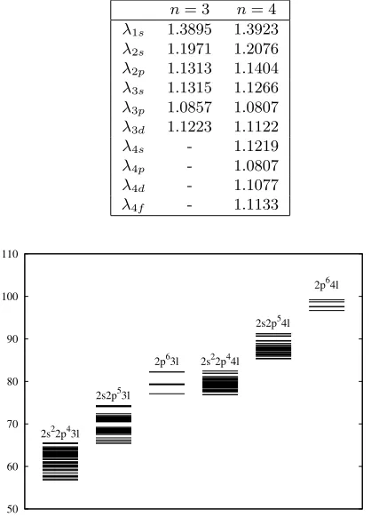
Table 1.Radial scaling factors used in AUTOSTRUCTURE to minimize the total energy of thenlorbital wave functions.

n= 3 n= 4

λ1s 1.3895 1.3923

λ2s 1.1971 1.2076

λ2p 1.1313 1.1404

λ3s 1.1315 1.1266

λ3p 1.0857 1.0807

λ3d 1.1223 1.1122

λ4s - 1.1219

λ4p - 1.0807

λ4d - 1.1077

λ4f - 1.1133

50 60 70 80 90 100 110

2s22p43l 2s2p53l

2p63l 2s22p44l 2s2p54l

2p64l

Fig. 1.Energy levels in Ry for both then= 3 (left) andn= 4 (right) structure calculations from AUTOSTRUCTURE.

given in Table I. Then= 3 energy levels are not changed

significantly by the addition of the n = 4 levels in the

larger calculation. The reason for this is demonstrated in

Figure 1 where the energy levels for the n = 4

calcula-tion are displayed. The only overlap between the n = 3

and n = 4 levels is between the 2p6₃

l and 2s2₂

p4₄

l els. Since only two-electron transitions connect these lev-els, this overlap does not have a significant effect on the energy levels. In Table II are listed the energies of the

lowest 66 levels from the n = 4 calculation compared to

those listed on the NIST website (Corliss & Sugar, 1982; http://physics.nist.gov). Since the level energies of the

n = 3 calculation are within 0.1% of the n = 4

calcu-lation they are not shown. With the exception of the first two excited states, which disagree by 2% and 1% respec-tively, all our level energies agree with the measurements of Corliss & Sugar to within 0.5%. We shall subsequently refer to levels using the energy ordered index given in this table.

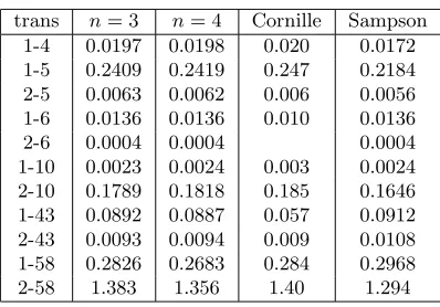
As a final test of the structure, we compare our os-cillator strengths with previous calculations. In Table III

are listed the oscillator strengths for both ourn= 3 and

n= 4-state calculations with a SUPERSTRUCTURE

cal-culation of Cornille et al. (1992) and the relativistic atomic structure calculation by Sampson et al. (1991). There is generally good agreement between all the calculations.

Both the n= 3 and n = 4 R-matrix calculations

clude the mass-velocity and Darwin corrections and in-clude a total of 20 continuum terms per channel. A

full-exchange calculation is performed forJ ≤10 and a

non-exchange calculation then provides the contribution up to

J = 38 and a further top-up is done using the Burgess sum

rule (see Burgess, 1974). In the outer region, we calculate the collision strengths up to an electron-impact energy of

200 Ry on a energy mesh with a spacing of 10−5_z2Ry in

regions with strong resonance contributions, a spacing of

10−4_z2Ry was used for the region between the_n= 2 and

n= 3 resonances, and a spacing of 10−3_z2Ry was used for

high energies outside the resonance region. Although this energy spacing does not resolve all resonances, the more than 15 000 energy points used are believed to to suffi-ciently sample the small width resonances as discussed by Badnell & Griffin (2001).

Effective collision strengths at high temperatures are obtained for dipole and Born allowed transitions by interpolation between the R-matrix calculation at 200 Ry and an infinte energy point calculated by AUTOSTRUCTURE.

3. Results

Overall, the differences between the n = 3 and n = 4

calculations are small. In Fig. 2, we compare the colli-sion strength of both calculations for the 1-4 transition.

While the n= 3 calculation shows stronger resonant

en-hancement for scattered electron energies below 3 Ry, the differences are not excessive. We also observe that the

ad-ditional n= 4 resonances for energies larger than 10 Ry

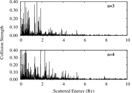
are small and not likely to have a large effect on the ef-fective collision strength. Similar features are seen for the 2-4 transition in Fig. 3.

To get a better measure of the resonant enhancement, we plot in Figures 4 and 5 the effective collision strengths for the 1-4 and 2-4 transitions respectively. Also included

in these figures is a reduced n = 3 R-matrix calculation

by Mohan et al. (1987) where the 2s2p5₃

land 2p6₃

lterms

are not included in the target expansion. In Fig. 4, there

is about a 10% difference between the present n= 3 and

n= 4 calculations while the Mohan et al. calculation is a

factor of four smaller at low temperatures and only coming within a factor of two at the highest temperatures shown. We see a similar disagreement between the Mohan et al. results and the present calculation in Fig. 5 for the 2-4 transition. In this case, however, the collision strength of

the n = 4 calculation is about 50% higher than that of

the n= 3 calculation at low temperatures, although the

absolute difference for this weak transition is about the same as in the 1-4 transition. Again, the effective collision strength from the Mohan et al. calculation is much smaller at low temperatures and coming into decent agreement at the end of the plotted temperature range. The difference

between the Mohan et al. calculation and ourn= 3

calcu-lation demonstrates the importance of the 2s2p5₃

l terms

on transitions involving the 2s2₂

p4₃

[image:4.595.52.545.80.344.2]

Table 2.Lowest 66 energy levels in Ry forn= 4 calculation compared to experimental measurements of Corliss & Sugar (1982) (see http://physics.nist.gov).

i Level Present NIST i Level Present NIST i Level Present NIST

1 2p5 2

P3o/2 0.0 0.0 23 2p

4₃

p2

So1/2 60.309 45 2p 4₃

d4

F7/2 63.111

2 2p5 2

P1o/2 0.955 0.935 24 2p 4

3p2

D3o/2 60.356 46 2p 4

3d2

D3/2 63.140

3 2s2p6 2

S1/2 9.830 9.702 25 2p 4

3p2

F5o/2 60.693 47 2p 4

3d4

P5/2 63.297 62.911

4 2p43s4P5/2 56.798 56.699 26 2p 4

3p2F7o/2 60.878 48 2p 4

3d2P3/2 63.418 63.308

5 2p43s2P3/2 57.052 56.937 27 2p 4

3p2D3o/2 61.016 49 2p 4

3d2D5/2 63.516 63.401

6 2p4₃

s4

P1/2 57.492 57.503 28 2p 4₃

p2

D5o/2 61.126 50 2p 4₃

d2

G7/2 63.787

7 2p4₃

s4

P3/2 57.664 57.573 29 2p 4₃

p2

P3o/2 61.590 51 2p 4₃

d2

G9/2 63.825

8 2p4

3s2

P1/2 57.899 57.798 30 2p 4

3p2

P1o/2 61.758 52 2p 4

3d2

F5/2 64.052

9 2p4

3s2

D5/2 58.444 31 2p 4

3d4

D5/2 62.114 53 2p 4

3d2

S1/2 64.056 63.919

10 2p43s2D3/2 58.478 58.355 32 2p 4

3d4D7/2 62.127 54 2p 4

3d2F7/2 64.156

11 2p4

3p4

P3o/2 59.019 33 2p 4

3d4

D3/2 62.157 55 2p 4

3d2

P3/2 64.280 64.139

12 2p4

3p4

P5o/2 59.053 34 2p 4

3d4

D1/2 62.247 56 2p 4

3d2

D5/2 64.335 64.160

13 2p43p4P1o/2 59.296 35 2p 4

3p2P3o/2 62.335 57 2p 4

3d2D3/2 64.558 64.391

14 2p43p4D7o/2 59.350 36 2p 4

3d4F9/2 62.356 58 2p 4

3d2P1/2 64.623 64.465

15 2p4₃

p2

D5o/2 59.365 37 2p 4₃

d2

F7/2 62.452 59 2p43d2D5/2 65.356 65.305

16 2p4₃

s2

S1/2 59.807 59.917 38 2p 4₃

p2

P1o/2 62.542 60 2s2p 5₃

s4

P5o/2 65.396

17 2p4

3p4

D1o/2 59.810 39 2p 4

3d4

P1/2 62.597 62.497 61 2p 4

3d2

D3/2 65.542 65.468

18 2p4

3p4

D3o/2 59.840 40 2p 4

3d4

P3/2 62.734 62.626 62 2s2p 5

3s4

P3o/2 65.726

19 2p43p2P1o/2 59.844 41 2p 4

3d2F5/2 62.816 63 2s2p 5

3s4P1o/2 66.140

20 2p43p2P3o/2 59.980 42 2p 4

3d2P1/2 62.957 64 2s2p 5

3s2P3o/2 66.221

21 2p43p4D5o/2 60.124 43 2p 4

3d4F3/2 62.989 65 2s2p 5

3s2P1o/2 66.709

22 2p4₃

p4

So3/2 60.157 44 2p 4₃

d4

F5/2 63.012 66 2s2p53p4S3/2 67.505

Table 3. Comparison of various calculated gf-values for present calculations with Cornille et al. (1992) and Sampson et al. (1991).

trans n= 3 n= 4 Cornille Sampson 1-4 0.0197 0.0198 0.020 0.0172 1-5 0.2409 0.2419 0.247 0.2184 2-5 0.0063 0.0062 0.006 0.0056 1-6 0.0136 0.0136 0.010 0.0136 2-6 0.0004 0.0004 0.0004 1-10 0.0023 0.0024 0.003 0.0024 2-10 0.1789 0.1818 0.185 0.1646 1-43 0.0892 0.0887 0.057 0.0912 2-43 0.0093 0.0094 0.009 0.0108 1-58 0.2826 0.2683 0.284 0.2968 2-58 1.383 1.356 1.40 1.294

The 1-4 and 2-4 transition comparisons are typical of the rest of the transitions with few exceptions. In some

cases, particularly for very weak transitions, the n = 4

resonant enhancement can dominate over the n = 3

res-onances. To illustrate this scenario, we show, in Fig. 6, a comparison of the 2-66 collision strength for both

calcu-lations Here we see, not only the strong, extended n= 4

resonant features in the larger calculation, but then= 4

calculation also has much stronger enhancement of the

n = 3 resonance contribution. Although not shown, the

n = 4 effective collision strength is a factor of 3 larger

than then= 3 calculation at logT = 6.2 and is twice as

large for logT = 7.0.

Using the ADAS suite of collisional-radiative modeling codes, we now explore how the differences seen between

the two calculations effect the prediction of observed

ra-diative emission of a low density Fe17+_{plasma. At an}

elec-tron temperature of 550 eV, the primary and secondary

emission peaks are at 14.2 and 16.0 ˚A respectively. Both of

these peaks are due ton= 3 levels exclusively. The largest

emission peak in the region where there are both n = 3

andn= 4 levels, occurring at 13.4 ˚A, is 15 times smaller

than the primary peak. In Figures 7, 8 and 9, we show the emission spectra for these three peaks. In addition to the spectra for the present calculations, we show the spectrum

from a modifiedn= 4 plane-wave Born calculation and a

hybrid spectrum which supplements the presentn= 3R

-matrix with then= 4 data from the modified plane-wave

Born calculation. The modified plane-wave Born calcula-tion is a standard plane-wave Born calculacalcula-tion (Burgess et al., 1997) which has been modified as to have a non-zero collision strength at threshold (see Cowan, p. 569). Starting with the primary peak in Fig. 7, we see that the

peak from the n = 4 calculation is about 25% smaller

than for then= 3 calculation. Then= 4 modified

plane-wave Born calculation severely overestimates the present

n = 4 calculation and the hybrid result closely matches

then= 3R-matrix calculation. In Fig. 8, we find that the

n = 4 peak is larger by about 35% over then= 3 peak.

Again, the modified plane-wave Born calculation misses

the mark having only half the intensity of the n = 4

R-matrix result. The hybrid result is found to improve

slightly over the n = 3 R-matrix calculation but is still

15% lower than the n = 4 spectra. Finally, in Fig. 9, we

examine the largest peak in the region where both the

[image:4.595.67.266.402.541.2]

4 M. C. Witthoeft et al.: Atomic Data from the IRON Project

0.0 0.2 0.4 0.6 0.8 1.0

0 5 10 15 20

Collision Strength

Scattered Energy (Ry)

n=4 n=3

0.0 0.2 0.4 0.6 0.8 1.0

0 5 10 15 20

[image:5.595.46.264.52.206.2]

n=4 n=3

Fig. 2.Collision strengths versus scattered electron energy for the n = 3 (top) and n = 4 (bottom) calculations of the 1-4 transition.

0.00 0.10 0.20 0.30 0.40

0 2 4 6 8 10

Collision Strength

Scattered Energy (Ry) n=4 n=3

0.00 0.10 0.20 0.30 0.40

0 2 4 6 8 10

[image:5.595.309.518.52.206.2]

n=4 n=3

Fig. 3.Collision strengths versus scattered electron energy for the n = 3 (top) and n = 4 (bottom) calculations of the 2-4 transition.

hybrid spectrum does a good job reproducing then = 4

R-matrix spectrum. The modified plane-wave Born

calcu-lation is too high while the n = 3 R-matrix calculation

is smaller than the n = 4 calculation. Taking all these

results into account, it appears that although the n = 4

plane-wave Born is a poor approximation for these spectra

at all wavelengths, the smallern= 3R-matrix calculation

supplemented by then= 4 Born calculation does perform

well in the region where bothn= 3 andn= 4 resonances

exist and does no worse than the n= 3 R-matrix

calcu-lation alone where there is only emission from then= 3

resonances. By extension, we would expect similar results

from a hybrid data set composed of the n= 4R-matrix

calculation and an n = 5 modified plane-wave Born

cal-culation, although this would need to be investigated.

4. Summary

TwoR-matrix calculations in intermediate coupling were

performed for electron-impact exctitation of Fe17+_{. The}

effective collision strengths of then= 4 calculation have

been archived for all 38 781 transitions, expanding on

0.00 0.01 0.02 0.03 0.04 0.05

6.2 6.4 6.6 6.8 7.0

Eff. Collision Strength

log T

[image:5.595.47.264.262.414.2]

1-4

Fig. 4.Effective collision strengths of the 1-4 transition com-paring the present n= 3 calculation (solid),n= 4 calculation (dashed) and an n= 3 R-matrix calculation by Mohan et al. (1987).

0.000 0.002 0.004 0.006 0.008 0.010

6.2 6.4 6.6 6.8 7.0

Eff. Collision Strength

log T

2-4

Fig. 5.Effective collision strengths of the 2-4 transition com-paring the present n= 3 calculation (solid),n= 4 calculation (dashed) and an n= 3 R-matrix calculation by Mohan et al. (1987).

the work done in IP XXVIII (Berrington et al., 1998). Differences of 10-20% in the effective collision strengths

between the smaller n = 3 calculation and the extended

n = 4 calculation persist for the majority of the

transi-tions. The addition of the 2s2p5₃

l and 2p6₃

l terms in the

presentn= 3R-matrix calculation are found to have

sig-nificant effects on the collision strengths to the 2s2₂

p4₃

l

levels when compared the the R-matrix calculation of

Mohan et al. (1987). The ADAS suite of collisional ra-diative modeling codes were used to obtain spectra from

a low-density Fe17+

plasma at an electron temperature of 550 eV. The differences found in the collision strengths

between the twoR-matrix calculations translate to the

in-tensity peaks of the emission spectra. The spectrum from a modified plane-wave Born calculation performs poorly at all wavelengths investigated but a hybrid spectrum

com-posed of then= 3R-matrix calculation supplemented by

the n= 4 modified plane-wave Born calculation is found

[image:5.595.306.518.276.430.2]

0.000 0.010 0.020 0.030 0.040

0 5 10 15 20

Collision Strength

Scattered Energy (Ry) n=4 n=3

0.000 0.010 0.020 0.030 0.040

0 5 10 15 20

[image:6.595.47.264.51.206.2]

n=4 n=3

Fig. 6.Collision strengths versus scattered electron energy for the n= 3 (top) andn= 4 (bottom) calculations of the 2-66 transition.

0.0 10.0 20.0 30.0 40.0 50.0 60.0 70.0 80.0

14.0 14.2 14.4 14.6 14.8 15.0

Intensity (Arbitrary Units)

Wavelength (Angstroms) n=3 n=4 mod. Born hybrid

Fig. 7. Radiative emission from a collisional radiative model (ADAS) in the low denisty limit at an electron temperature of 550 eV for a wavelength range of 14.0 to 14.6 ˚A. Then= 3 calculation is the dotted curve,n = 4 is the solid curve, the dashed curve shows the modified plane-wave Born calculation from AUTOSTRUCTURE, and the hybridR-matrix/Born re-sult is shown as the dot-dash curve.

alone, especially in regions where both n= 3 and n= 4

resonances contribute.

Acknowledgements. One of us (MCW) would like to thank Allan Whiteford for his help in running the ADAS colli-sional radiative modeling codes. This work has been funded by PPARC grant PPA/G/S2003/00055.

References

ADAS web page: http://adas.phys.strath.ac.uk

Badnell, N. R. 1986, J. Phys. B: At. Mol. Phys., 19, 3827 Badnell, N. R. & Griffin, D. C. 2001, J. Phys. B: At. Mol. Opt.

Phys., 34, 681

Berrington, K. A., Saraph, H. E., Tully, J. A. 1998, A&AS, 129, 161 (IP XXVIII)

Burgess, A. 1974, J. Phys. B: At. Mol. Phys., 7, L364 Burgess, A., Chidichimo, M. C., Tully, J. A. 1997 J. Phys. B:

At. Mol. Opt. Phys., 30, 33

Corliss, C. & Sugar, J. 1982, J. Phys. Chem. Ref. Data, 11, 135

0.0 5.0 10.0 15.0 20.0 25.0 30.0 35.0 40.0 45.0

15.6 15.8 16.0 16.2 16.4

Intensity (Arbitrary Units)

Wavelength (Angstroms) n=3

[image:6.595.310.525.52.206.2]

n=4 mod. Born hybrid

Fig. 8. Radiative emission from a collisional radiative model (ADAS) in the low denisty limit at an electron temperature of 550 eV for a wavelength range of 15.5 to 16.4 ˚A. Then= 3 calculation is the dotted curve, n= 4 is the solid curve, the dashed curve shows the modified plane-wave Born calculation from AUTOSTRUCTURE, and the hybridR-matrix/Born re-sult is shown as the dot-dash curve.

0.0 0.5 1.0 1.5 2.0 2.5 3.0 3.5 4.0 4.5

12.6 12.8 13.0 13.2 13.4 13.6 13.8 14.0

Intensity (Arbitrary Units)

Wavelength (Angstroms) n=3

n=4 mod. Born hybrid

Fig. 9. Radiative emission from a collisional radiative model (ADAS) in the low denisty limit at an electron temperature of 550 eV for a wavelength range of 12.5 to 14.0 ˚A. Then= 3 calculation is the dotted curve, n= 4 is the solid curve, the dashed curve shows the modified plane-wave Born calculation from AUTOSTRUCTURE, and the hybridR-matrix/Born re-sult is shown as the dot-dash curve.

Cornille, M., Dubau, J., Loulergue, M., Bely-Dubau, F., Faucher, P. 1992, A&A, 259, 669

Cowan, R. D. 1981, The Theory of Atomic Structure and Spectra, (California: University of California Press), 569 Griffin, D. C., Badnell, N. R., Pindzola, M. S. 1998 J. Phys.

B: At. Mol. Opt. Phys., 31, 3713

Hummer, D. G., Berrington, K. A., Eissner, W., et al. 1993, A&A, 279, 298

Mann, J. B. 1983, At. Data Nuc. Data Tables, 29, 407 Mohan, M., Baluja, K. L., Hibbert, A., Berrington, K. A. 1987,

J. Phys. B: At. Mol. Phys., 20, 6319 NIST web page: http://physics.nist.gov

[image:6.595.46.265.260.414.2] [image:6.595.306.522.305.458.2]