Abstract—This paper presents a robust control algorithm based on adaptive proportional-integral-derivative (PID) controller and sliding mode control (SMC) approach. In this paper, the drawbacks of SMC are compensated by adopting an adaptive PID continuous second order sliding mode control approach (APID2SMC) with PID sliding surface. The stability of the system is guaranteed in the sense of Lyapunov theorem. Numerical simulations using the dynamic model of DC motor with modeling uncertainties show that the proposed approach provides robustness for trajectory tracking performance under the occurrence of uncertainties. These simulation results compared to the results of conventional sliding mode control (CSMC) and PID control approaches indicate that the proposed method yields superior performance than the other controllers.
Index Terms— robust control, second order sliding mode control
I. INTRODUCTION
LIDIN mode control (SMC) is one of the effective nonlinear robust control approaches since it provides system dynamics with an invariance property to uncertainties once the system dynamics are controlled in the sliding mode [4], [7]–[8], [11]–[12]. Under certain conditions, the SMC is robust with respect to system perturbation and external disturbance [4], [14]. However, this control strategy produces some drawbacks associated with large control chattering that may wear coupled mechanisms and excite undesirable high-frequency dynamics. Moreover, a priori knowledge of the upper bounds of the norm of the perturbation vector is required to obtain robustness and convergence. In order to overcome the drawbacks of SMC, the problem of perturbation estimation was investigated in [1] for a particular class of nonlinear uncertain systems. However, these problems remained mainly unsolved [9].
Several methods of chattering reduction have been reported. One approach [5] places a boundary layer around the switching surface such that the relay control is replaced by a saturation function. Another method [13] replaces a max–min-type control by a unit vector function. These approaches, however, provide no guarantee of convergence
Wael M. Elawady is with faculty of Engineering, Tanta University, Egypt (corresponding author to provide phone: 0201026655098; e-mail:wmeana2007@ yahoo.com).
Samar A. Lebda is with faculty of Engineering, Tanta University, Egypt (e-mail:[email protected]).
Amany M. Sarhan is with faculty of Engineering, Tanta University, Egypt (e-mail: [email protected]).
to the sliding mode and involve a tradeoff between chattering and robustness. In [6], an asymptotic observer in the control scheme can eliminate chattering despite the discontinuous control law. Both the boundary layer approach and the observer design assume that the un-modeled dynamics are completely unknown. In [2], the authors use the integral sliding method to overcome the drawback of chattering phenomenon. The authors in [10] attempted to reduce the well-known chattering problem in classical sliding mode control by presenting an innovative approach to adaptive fuzzy sliding mode control for a class of single input single output continuous nonlinear systems with unknown dynamics and bounded disturbances. In [14], a chattering free adaptive sliding mode controller is proposed for stabilizing a class of multi-input multi-output (MIMO) systems affected by both matched and mismatched types of uncertainties.
This paper discusses the design of a robust adaptive PID continuous second order sliding controller (APID2SMC) with PID sliding surface to achieve system robustness against parameter uncertainty, external load disturbance, and nonlinearities. In this approach, different from the second order sliding mode control presented in [3], an adaptive PID controller with on line tuned parameters replaces the equivalent control term which is not used because it needs exact full system dynamics knowledge and the discontinuous term is replaced by a PD control in terms of sliding surface dynamics. The proposed approach has some features such as a priori knowledge of the bounds of uncertainties is not required and the chattering phenomenon is eliminated without deteriorating the system robustness. The stability of the system is guaranteed in the sense of the Lyapunov stability theorem.
The proposed control algorithm is applied to a speed control of DC motor through simulations. The proposed approach is compared to the existing conventional controllers. The simulation results indicate that the control performance of the proposed control strategy is satisfactory and better than those of the existing conventional controllers. The remainder of this paper is organized as follows: section II presents the proposed adaptive PID second order sliding mode control. Section III presents the stability of the system in the sense of Lyapunov stability theorem. Section IV presents the simulation results, and section V summarizes the conclusions and contributions of the work
Continuous Second Order Sliding Mode Control
With On Line Tuned PID
Wael M. Elawady, Samar A. Lebda and Amany M. Sarhan
II. ADAPTIVEPIDSECONDORDERSLIDINGMODE CONTROL
The main objective in this paper is to adopt an adaptive PID-based second order sliding mode control approach (APID2SMC) in which: (i) the equivalent control term in [3] is replaced by an on line tuned adaptive PID controller which results in more robustness, fast dynamic response and good steady state accuracy. (ii) the discontinuous control in [3] is replaced by a continuous proportional derivative (PD) controller in terms of sliding surface dynamics which completely eliminates the requirement of a priori knowledge of the bounds of uncertainties and the chattering effects.
The dynamics of a single-input linear uncertain plant can be written as [3]:
y(t)ay(t)by(t)cu(t)D(t)
(1) where y(t) is the output, u(t) is the control input and d(t)
represents the disturbances and un-modeled dynamics. a, b and c are plant parameters. In general, the system
parameters involve a nominal part and some variations, therefore, in the presence of the model uncertainties and
external disturbances, (1) can be written as follows:
) ( ) ( ) (
) ( ) ( ) ( ) ( ) (
t D t u c c
t y b b t y a a t y
(2) It is assumed that all uncertain elements can be lumped as follows:
) ( ) ( ) ( ) ( )
(t ayt byt cut Dt
D
(3) The dynamics of the model is written as:
) ( ) ( ) ( ) ( )
(t ay t byt cu t Dt y
(4) The second order sliding PID surface in the space of tracking error can be defined as [3]:
s(t) s(t) e(t) 1e(t) 2 e( )d
(5) where e(t) y(t)yd(t) is the tracking error, in which
) (t
yd is the desired output. 1, 2 and are positive constants.
The tracking control problem can be achieved by keeping the system trajectory on the sliding surface s(t)0. For
this purpose, the proposed control algorithm is chosen as:
() ()
1 )
( u t u t
c t
u PID a
(6) where uPID(t) and ua(t) are the adaptive PID control with online tuned gains and the continuous PD control, respectively.
The adaptive PID control law uPID(t)
can be chosen as:
() () ( ) ()
^ ^
^
t e k d e k t e k t
uPID p i d
(7) where kp
^ , ki
^
and kd
^
are the adaptive proportional, integral and derivative gains to be tuned online.
The continuous proportional derivative (PD) control law, )
(t
ua , can be chosen as: ) ( ) ( )
(t kst D t
u
(8)
where k is a positive constant which is a design parameter
and Dest(t) is the estimated perturbation.
III. LYAPUNOVSTABILITYANALYSIS Lyapunov stability analysis is the most popular approach to prove and evaluate the stable convergence property of sliding mode control. Here, Lyapunov stability approach is employed to investigate the stability property of the proposed controller. Lyapunov function can be chosen as:
2 ~ 2 ~
2 ~ 2
~ 2
2
2 1 2
1
2 1 ) ( 2
1 ) ( 2 1 ) ( 2 ) (
i i d d
p p D
k k
k t
D t
s t s t V
(9)
where D, p, d and i are positive constants which are design parameters and D~ is the lumped uncertainty
estimation error and is defined as follows [9]: ( ) ( ) ( )
~
t D t D t
D est
(10) ~
p
k ,
~
d
k and
~
i
k are the deviations between the adaptive PID
gains and initial gains and are defined as: i i i d d d p p
p k k k k k k k k
k
^ ~ ^
~ ^
~
, ,
(11) where kp, ki and kd are the initial proportional, integral and derivative gains
The derivative of Lyapunov function is:
i i i
d d d p p p D
k k
k k k k D D s s t s s t V
~ ~
~ ~ ~ ~ ~ ~
1
1 1
1 )
( ) (
(12)
Take the derivative of surface in (5) with respect to time and use (4), then
d d
y D t u c y b y a s e e
s e e y y s e e e t s
) ( )
(
2 1
2 1 2
1
(13)
Substituting (13) into (12) yields
i i i d d d p p p D
d
k k k k k k D D
y D t u c y b y a s e e s s s t V
~ ~ ~ ~ ~ ~ ~ ~
2 1
1 1
1 1
} )
( {
) (
(14)
By substituting (7) and (8) into (6), the proposed controller
)
(
t
u
is chosen as:)} ( ) ( ) ( )
(
) ( { 1 )} ( ) ( { 1 ) (
^ ^
^
t D t s k t e k d e k
t e k c t u t u c t u
est d
i
p a
PID
(15)
i i i d d d p p p D d est d i p k k k k k k D D y D D s k e k d e k e k y b y a s e e s s s t V
~ ~ ~ ~ ~ ~ ~ ~ ^ ^ ^ 2 1 1 1 1 1 } ) ( { ) (
(16)Substituting yeyd and y e yd
into (16) yields
i i i d d d p p p D d est d i p d d k k k k k k D D y D D s k e k d e k t e k y e b y e a e e s s s s t V
~ ~ ~ ~ ~ ~ ~ ~ ^ ^ ^ 2 1 1 1 1 1 } ) ( ) ( ) ( ) ( { ) ( (17)Rearranging (17) gives:
i i i d d d p p p D d est d i p d d k k k k k k D D y D D s k e k d e k e k y b y a e b e a s s s s t V
~ ~ ~ ~ ~ ~ ~ ~ ^ ^ ^ 2 1 1 1 1 1 } ) ( ) ( ) ( { ) ( (18)Differentiating (10) and (11) and substituting in (18) yields:
i i i d d d p p p est D d est d i p d d k k k k k k D D y D D s k e k d e k e k y b y a e b e a s s s s t V
^ ~ ^ ~ ^ ~ ~ ^ ^ ^ 2 1 1 1 1 1 } ) ( ) ( ) ( { ) ( (19)Using (10), (19) can be written as:
i i i d d d p p p est D d i p d d d k k k k k k D D s e k d e k s s e k D s s k y y b y a e b e a s s s s t V
^ ~ ^ ~ ^ ~ ~ ^ ^ ^ ~ 2 1 1 1 1 1 ) ( } ) ( ) ( { ) ( (20)Rearranging (20) gives:
i i i d d d p p p d i p est D d d d k k k k k k s e k d e k s s e k D D D s s k e b e a y b y a y s s s s t V
^ ~ ^ ~ ^ ~ ^ ^ ^ ~ ~ 2 2 1 1 1 1 ) ( 1 } ) ( ) ( { } { ) (
(21)Using (11), (21) can be manipulated as:
i i i d d d p p p d d i i p p est D d d d k k k k k k s e k k d e k k s s e k k D D D s s k e b e a y b y a y s s s s t V
^ ~ ^ ~ ^ ~ ~ ~ ~ ~ ~ 2 2 1 1 1 1 ) ( ) ( ) ( ) ( 1 } ) ( ) ( { } { ) ( (22) i i i d d d p p p d d i i p p est D d d d k k k k k k s e k s e k d e k s d e k s s e k s e k D D D s s k e b e a y b y a y s s s s t V
^ ~ ^ ~ ^ ~ ~ ~ ~ ~ ~ 2 2 1 1 1 1 ) ( ) ( 1 } ) ( ) ( { } { ) ( (23)From (5), (23) can be rewritten as:
d d d d i i i i p p p p d i p est D d d d k k s e k k k d e k s k k s e k s e k d e k s s e k s D D s k e b e a y b y a y s s d e e e s s t V
^ ~ ~ ^ ~ ~ ^ ~ ~ ~ 2 2 1 2 1 1 1 ) ( 1 ) ( ) 1 ( } ) ( ) ( { } ) ( { ) ( (24) ) ) ( 1 ( ) ) ( 1 ( ) 1 ( ) 1 ( ) ( } ) ( ) ( { } ) ( { ) ( ^ ~ ^ ~ ^ ~ ~ 2 2 1 2 1
s t e k k d e s k k s e k k s D D s e k d e k s s e k s k e b e a y b y a y s s d e e e s s t V d d d i i i p p p est D d i p d d d (25)Rearranging (25) yields:
) 1 ( ) ( 1 ( ) 1 ( ) 1 ( } { } ) ( ) ( ) ( ) 1 {( ) 1 ( ) ( ^ ~ ^ ~ ^ ~ ~ 2 2 1 1 2
s e k k d e s k k s e k k s D D y b y a y s d e k e k b e k a s s k t V d d d i i i p p p est D d d d i p d (26)For V(t)0, the updated laws of the adaptive PID controller gains can be written as:
et s k s
e d k et s kp p() , i i ( ) , d d ()^ ^ ^ (27) The time evolution of the estimated uncertainty Dest(t) is
chosen as:
s
t
D
est(
)
D (28)} {
} ) ( ) (
) (
) 1 {( ) 1 ( ) (
2
2 1 1
2
d d d i
p d
y b y a y s d e k
e k b e
k a s s k t V
(29)
For V(t)0, the following conditions must be satisfied: kd 1a1, kp 12b, ki 2 (30) Substituting (30) into (29) yields
} {
) 1 ( ) (
} {
) 1 ( ) (
2 2
d d d
d d d
y b y a y s s k t V
y b y a y s s k t V
(31)
From the above analysis the global asymptotic stability is guaranteed since V(t)0. From (6), (7), (8) and (28), the total proposed robust adaptive controller is expressed as:
)]} ( ) ( [
)] ( )
( ) ( {[ 1 ) ( ) ( 1 )
( ^ ^ ^
t s t s k
t e k d e k t e k c t u t u c t u
D
d i
p a
PID
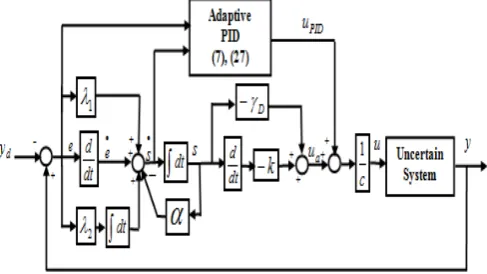
(32) [image:4.595.48.292.57.322.2]where the adaptive gains of PID term are defined in (27). The block diagram of the proposed control approach is depicted in Fig. 1.
Fig. 1. Block diagram of adaptive PID second order sliding mode control
IV. SIMULATIONRESULTS
[image:4.595.52.296.374.511.2]The proposed approach was tested for the speed control of the DC motor shown in Fig. 2 to validate the feasibility and effectiveness of the presented control algorithm.
Fig. 2. DC motor model
The dynamics of DC motor are given by: ) ( ) ( ) ( ) ( )
(t awt bwt cut Dt
w
where w represents speed,
a a
L R J B
a ,
a t b a
JL k k BR
b and
a t
JL k
c . u(t)Ea represents the motor armature voltage,
1.6 a
R , La 0.1H represent the armature coil
resistance and inductance, respectively, 2
/ / . 1 .
0 Nm rad s
J is the moment of inertia,
s rad m N
B0.5 . / / represents coefficient of viscous
friction, kt 0.1N.m/A represents the torque constant and
. / . / 1 .
0 V rad s
kb represents the back emf constant. All
simulations are carried out using MATLAB R2009b. In order to show the effectiveness and robustness of the proposed approach, large severe uncertainties D(t) are
occurred which contains:
1. A step external load disturbance torque of 5N.m is
suddenly applied at the motor shaft at t1.0 s. and is shown in Fig. 3.
0 0.2 0.4 0.6 0.8 1 1.2 1.4 1.6 1.8 2 0
1 2 3 4 5
Time (sec.)
E
xt
er
nal
loa
d
di
st
ur
ba
nc
e
to
rq
ue
Fig. 3. External load disturbance torque 2. An unpredicted variation of the armature resistance
a
R and coefficient of viscous friction Boccurred
at t1.0 s. The abrupt changes of Ra and B are
shown in Fig. 4.
0 0.2 0.4 0.6 0.8 1 1.2 1.4 1.6 1.8 2 1.2
1.4 1.6 1.8 2 2.2 2.4
Time (sec.)
A
rm
atu
re
r
es
is
tn
ce
(a) Armature coil resistance
0 0.2 0.4 0.6 0.8 1 1.2 1.4 1.6 1.8 2 0.4
0.45 0.5 0.55 0.6 0.65 0.7 0.75 0.8
Time (sec.)
C
oe
ffi
ci
en
t o
f v
is
co
us
fr
ic
tio
n
(b) Coefficient of viscous friction
[image:4.595.65.276.601.741.2]Simulations are performed in the case of set-point tracking in which the command desired motor speed is set equal to 500rpm. For comparison, conventional PID
controller and conventional sliding mode control (CSMC) are used.
The parameters of the proposed APID2SMC are set as: 50
, 12, 2 1, k20, D 10, p 0.5, 08
. 0
i
and d 0.01.
Fig. 5 shows the DC motor speed response profile. The time history of the sliding surface s(t) for CSMC is
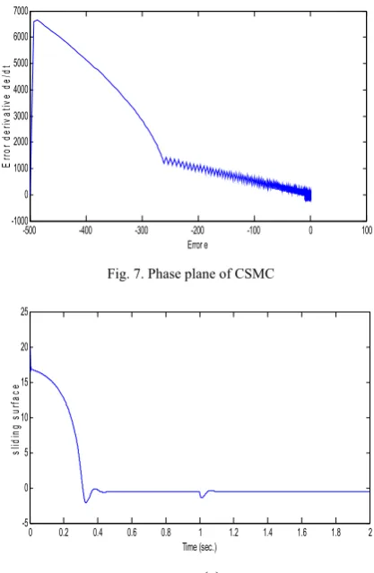
depicted in Fig. 6. The phase portrait trajectory for CSMC is shown in Fig. 7. The time history of the sliding surface s(t)
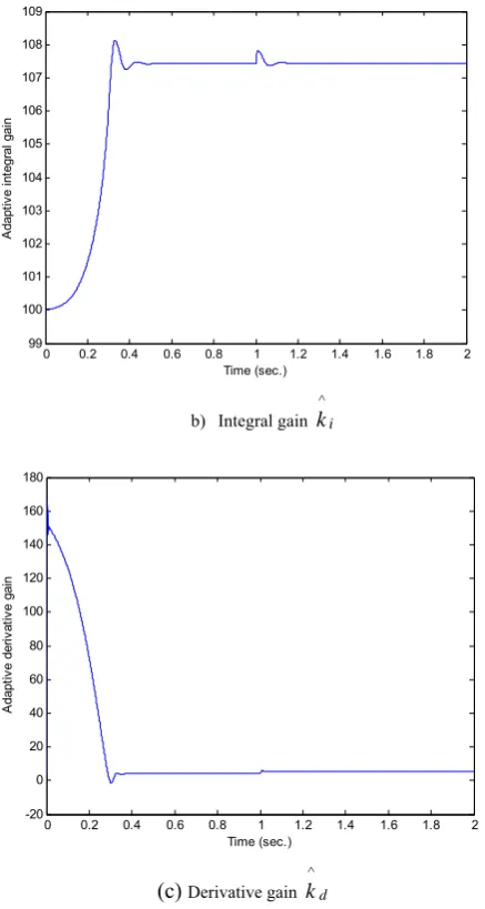
for APID2SMC is depicted in Fig. 8. The phase portrait trajectory for APID2SMC is shown in Fig. 9. The trajectory of the adaptive proportional gain kp
^
, adaptive integral gain i
k
^
and adaptive derivative gain kd
^
[image:5.595.171.514.53.748.2]defined in (27) for APID2SMC is shown in Fig. 10.
Fig. 5. Motor speed response
0 0.2 0.4 0.6 0.8 1 1.2 1.4 1.6 1.8 2 -5
0 5 10
Time (sec.)
sl
idi
ng
sur
fac
e
s(
t)
Fig. 6. Trajectory of s(t)of CSMC
-500 -400 -300 -200 -100 0 100
-1000 0 1000 2000 3000 4000 5000 6000 7000
Error e
E
rro
r
de
riv
at
iv
e
de
/d
[image:5.595.320.529.55.375.2]t
Fig. 7. Phase plane of CSMC
0 0.2 0.4 0.6 0.8 1 1.2 1.4 1.6 1.8 2
-5 0 5 10 15 20 25
Time (sec.)
slid
in
g
su
rf
ac
e
Fig. 8. Trajectory of
s
(
t
)
of APID2SMC-5 0 5 10 15 20 25
-3000 -2000 -1000 0 1000 2000
sliding surface s(t)
sl
idi
ng
sur
fac
e
der
iv
at
iv
e
ds
/dt
Fig. 9. Phase plane of CSMC
0 0.2 0.4 0.6 0.8 1 1.2 1.4 1.6 1.8 2
0 200 400 600 800 1000 1200 1400
A
dapt
iv
e
proprt
iona
l gai
n
Time (sec.)
a) Proportional gain kp
^
[image:5.595.56.287.314.691.2]0 0.2 0.4 0.6 0.8 1 1.2 1.4 1.6 1.8 2 99
100 101 102 103 104 105 106 107 108 109
A
dapt
iv
e
int
eg
ral
gai
n
Time (sec.)
b) Integral gain ki
^
0 0.2 0.4 0.6 0.8 1 1.2 1.4 1.6 1.8 2
-20 0 20 40 60 80 100 120 140 160 180
Time (sec.)
A
dapt
iv
e
der
iv
at
iv
e
gai
n
(c) Derivative gain kd
^
Fig. 10. Trajectory of adaptive gainsof APID2SMC
From the simulation results, it is concluded that the proposed approach (APID2SMC) showed superior performance. It is obvious that CSMC suffers from the chattering phenomenon; however, the proposed controller can eliminate the chattering phenomenon and yields favorable tracking response. The proposed approach provides perfect tracking under highly severe uncertainties and external disturbances. The proposed control law shows much less error than CSMC and PID control systems when comparing the results. Table I shows performance indices computed for each of the different controllers. The performance indices are integral of absolute error (IAE) and integral time multiplied absolute error (ITAE) given by:
e t dt ITAE t e t dt
[image:6.595.58.277.59.469.2]IAE () , () (34)
Table I Performance indices of different controllers
Algorithm IAE103 ITAE103
PID 121.9 165.9
CSMC 6.419 7.713
APIDSMC 3.669 3.294
V. CONCLUSION
The presented paper has presented an adaptive PID continuous second order sliding mode control methodology (APID2SMC) with PID sliding surface to achieve system robustness against parameter uncertainty and external load disturbance. In this approach, an adaptive PID controller with parameters being updated online replaces the equivalent control term and the discontinuous term is replaced by a continuous PD control in terms of sliding surface dynamics.
The proposed control algorithm has some features such as a priori knowledge of the bounds of uncertainties is not required and the chattering phenomenon is eliminated without deteriorating the system robustness. The closed-loop system is globally stable in the Lyapunov sense and the system output can track the desired output asymptotically in the presence modeling uncertainties and disturbances. Simulation results have showed that the performance of the proposed controller is better than the conventional approaches and has superior tracking performance with robust characteristics to conventional methods.
REFERENCES
[1] H. Elmali, N. Olgac, “Theory and implementation of sliding mode control with perturbation estimation”, IEEE Int. Conf. Robotics
Autom., pp. 2114–2119, 1992.
[2] H. F. Ho, Y. K. Wong, A. B. Rad, “Robust fuzzy tracking control for robotic manipulators," Simulat. Model. Pract. Theory vol. 15, pp.
801–816, 2007.
[3] I. Eker, " Second- order sliding mode control with experimental application", ISA Trans., vol. 49, no. 3, pp. 394-405, 2010. [4] J. J. E. Slotine and W. Li, Applied Nonlinear Control. Englewood
Cliffs, NJ: Prentice-Hall, 1991.
[5] J. J. Slotine and S. S. Sastry, “Tracking control of nonlinear systems using sliding surfaces, with application to robot manipulators”, Int.
J. Control, vol. 38, pp. 465–492, 1983.8
[6] J. Phuah, J. Lu, T. Yahagi, “Chattering free sliding mode control in magnetic levitation system”, IEE J. Trans. Electron. Inf. Syst. vol. 125, pp. 600-606, 2005.
[7] K. J. Astrom and B. Wittenmark, Adaptive Control. Reading, MA:
Addison-Wesley, 1995.
[8] K. K. Shyu and H. J. Shieh, “A new switching surface sliding-mode speed control for induction motor drive systems”, IEEE Trans.
Power Electron., vol. 11, pp. 660–667, Jul. 1996.
[9] M. Zeinali and L. Notash, "Adaptive sliding mode control with uncertainty estimator for robot manipulators", Mechanism and
Machine Theory, vol. 45, no. 1, pp. 80-90, 2010.
[10] O. Cerman and P. Hušek, "Adaptive fuzzy sliding mode control for electro-hydraulic servo mechanism", Expert Systems with
Applications, vol. 39, pp. 10269-10277, 2012.
[11] R. J. Wai, “Adaptive sliding-mode control for induction servo motor drive”, in Proc. Inst. Elect. Eng. Electr. Power Appl., vol. 147, no. 6, pp. 553–562, 2000.
[12] S. Aloui, et al., “Improved fuzzy sliding mode control for a class of MIMO nonlinear uncertain and perturbed systems”, Appl. Soft
Comput. J., vol. 11, pp. 820-826, 2010.
[13] S. K. Spurgeon “Choice of discontinuous control component for robust siding mode performance”, Int. J. Control, vol. 53, pp. 161– 179, 1991.