Abstract— There has been an increase in application of pendulum in robotics which is applicable in Medicine, Agriculture, Military, Industries Explorations and Entertainment. Many Researchers have shown interest in inverted pendulum stability and control in recent years. This study is concerned with the development of equation of motion of inverted pendulum and its analysis by adopting the Lagrangian and Differential Transform Method (DTM) respectively. The resulting equations were solved analytically. Results obtained are consistent with the ones in the literature. Index Terms—Applied Mechanics, Dynamics Differential transform method. Inverted pendulum, Lagrangian.
I. INTRODUCTION
N ordinary pendulum is one with the pivot at the top and the mass at the bottom. An inverted pendulum is the opposite way round. The pivot is at the bottom and the mass is on top. The inverted pendulum is a mechanism for carrying an object form one place to another and this is how it functions during walking. The ―passenger unit‖ as Perry would call it is carried forward by the outstretched leg as it pivots over the foot [1]. So an inverted pendulum is a pendulum that has its centre of mass above its pivot point. It is often implemented with the pivot point mounted on a moving body that can move horizontally. Unlike a normal pendulum which is always stable when hanging downwards, an inverted pendulum is inherently unstable, and must be actively balanced in order to remain upright. This can be done in different ways including the pivot point horizontally as part of a feedback system [2,3]. A simple demonstration of this is achieved by balancing an upturned broomstick on the end of
Manuscript received March 30, 2017; revised April 10, 2017.. This work was supported in full by Covenant University. Dynamic Modeling and Analysis of Inverted Pendulum using Lagrangian-Differential Transform Method
M.C. Agarana is with the Department of Mathematics, Covenant University,Nigeria,+2348023214236,michael.agarana@covenantu niversity.edu.ng
O.O. Ajayi is with the Department of Mechanical Engineering, Covenant University, Nigeria
one's finger. The inverted pendulum is a classic problem in dynamics and control theory and is used as a benchmark for testing control strategies[3,4]. Differential transform method is a semi analytical method which requires no discretization [4,5]. One of the advantages of DTM over others is that it is simple to apply [5,6,7]. The solution of the governing equation is very close to the analytical solutions [8]. The Lagrangian is a mathematical function of the generalized coordinates, their time derivatives, and time. It contains information about the dynamics of the system. Lagrangian mechanics is ideal for systems with conservative forces and for bypassing constraint forces in any coordinate system. Dissipative and driven forces can be accounted for by splitting the external forces into a sum of potential and non-potential forces [9]. When Newton's formulation of classical mechanics is not convenient, Lagrangian mechanics is widely used to solve mechanical problems in physics and engineering. Lagrangian mechanics applies to the dynamics of particles, and used in optimisation problems of dynamic systems. Lagrangian mechanics uses the energies (both kinetic and potential) in the system instead of forces. Thus a function that summarizes the dynamics of an entire system is simply known as the Lagrangian. Moreover, the Kinetic energy reflects the energy of the system's motion. The potential energy of the system reflects the energy of interaction between the particles, i.e. how much energy any one particle will have due to all the others and other external influences.[9]
The purpose of this study was to use differential transformation algorithm to solve the ordinary second order differential equation resulted from the deployment of Lagrangian to model the Kinematics of motion of inverted pendulum. DTM was then applied to solve the model so formed.[9] The dynamic effects of the pendulum through its angular displacement, angular velocity and
Dynamic Modeling and Analysis of Inverted
Pendulum using Lagrangian-Differential
Transform Method
Michael C. Agarana, Member, IAENG, and Oluseyi O. Ajayi
angular acceleration were estimated over a period of time.
[image:2.595.81.275.108.229.2] [image:2.595.59.281.270.379.2]
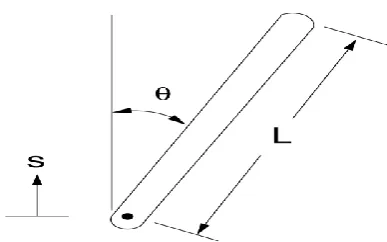
Fig. 1 The angular displacement of the inverted pendulum
Fig. 2 The vertical and horizontal components of the length of the inverted pendulum
Fig. 1 represents an inverted pendulum, while Fig. 2 is the schematic of the inverted pendulum, showing the vertical and horizontal components of the length of the inverted pendulum. represents the angle the inverted pendulum makes with the vertical.
II. EQUATION OF MOTION
Using Lagrange's equations, which employ a single scalar function rather than the vector components, to derive the equations modeling an inverted pendulum, we take partial derivatives. In classical mechanics, the natural form of the Lagrangian is defined as
L = Ek – Ep (1)
Where EK and EP are kinetic and potentialenergies
are respectively. Ep is defined by its mass m, and
the gravitational constant g:
Ep = mgh (2)
The kinetic energy Ek of a point object is defined by its mass m and velocity v:
Ek = 1/2mv2 (3)
Equation of motion can be directly derived by substitution using Euler Lagrange equation:
d L L
dt
(4)
where is the angle the pendulum makes with the upward vertical.
Equation (2) can be written as
Ep =mgy (5)
Where h = y, is the height along vertical axis From the figures 2a and 2b above,
x = Lsin (6) y = Lcos (7)
implies
This
dx Lcos ( ) d (8)
dt dt
sin ( ) (9)
equation (1), the Lagrangian can be written as
and
dy d
L
dt dt
From
2
2 2
2
1
L = mv - mgy (10) 2
where h = y
Velocity as a vector quantity is given as
v = dx + dy
dt dt
2 2
2 2 2 2 2
(11) Substituting equations (6) and (7) into
equation (11) gives:
v = L d cos L d sin (12)
dt dt
2
2 2 2 2
2 2 2
v = L cos sin (13)
v = L (14)
Now substituting equations (7) and (14) into equation ( d dt d dt 2 2 10) gives: 1
L = cos (15) 2 d mL mgL dt 2 which implies
sin (16)
(17) ( ) L mgL L d mL d dt dt 2 2 2 2 2 2 (18) ( )
Substituting equation (16) and (18) into equation (4) gives:
sin (19) T
d L d
mL d dt dt dt d mL mgL dt herefore 2
2 sin (20)
d g
dt L
Without oscillator and taking g =10 and L =5 gives:
'
( ) 2 sin (21) subject to
(0) = 0, (0) 2 (22)
t
III MODEL SOLUTION
To solve equation (20), is solved for using Differential transform method (DTM). However equation (20) is a linear second order differential equation solvable by applying differential transform method.
A. Differential Transformation Method (DTM)
Differential transform method is a numerical method based on Taylor expansion. This method tries to find coefficients of series expansion of
unknown function by using the initial data on the problem. The concept of differential transform method was first proposed by Zhou [10,11].
B. Definitions and Properties of DTM
With reference to article [4, 5, 6] the differential transformation of a function f(x) can be written as:
1 ( )
( ) 0 (23)
!
k
d f x
F t x
K dx
Where f(x) is referred to as the original function and F(x), the transformed function. The differential inverse of F(t) is
0
( ) ( ) k (24)
k
f x F t x
Equation (26) is the Tailor series expansion of f(x) about x=0. It can also be written as
0
( )
( ) (25)
!
k k
k
x d f x
f x k dx
Some operational properties of DTM are as follows:
i If f(x) = p(x) g(x), then F(t) = p(t) F(t) (26)
If f(x) = cp(x), then F(t) = cP(t), where c is a constant. (27)
( ) ( )!
If f(x) = , then F(t) = ( ) (28)
If f(x n
n
ii
d p x k n
iii p k n
dx k
iv
) = sin(ax + b), then F(x) = sin (29)
! 2
f(x) = e , ( ) , is a constant (30) ! k k x a k b k
v then F t where k
C. Differential Transform Method on Second Order ODE)
Second order linear differential equations can be used as follows [4]
2 1
( ) [ ( ) ( ) ]
f x r x cy x by x
a
(31)
1
( 2) [ ( ) ( 1) ( 1) ( )]
( 1)( 2)
F k R x b k F k cF k
a k k
(32)
which is subject to the initial condition that:
F(0) = F0 = a1 and F1(0) = F(1) = a2 (33)
Equation (33) is called recursive formula.
Using equation (33) on equation (32) gives the appropriate solution.[4]
IV. APPLICATION OF DTM
To apply the discussed DTM to equation (20), equations (32) and (33) are re-written as:
DT[ ( ) t 2sin ] (34)
'
( 1)( 2) ( 2) 2sinY(k) (35)
1
Y(k+2) = [2sin ( )] (36)
( 1)( 2)
with the initial conditions that Y(0) = 0, Y (0) = -2.
k k Y k
Y k
k k
(37) Applying the recursive relation in (33) with
0
k the values for Y(2), Y(3), Y(4), …, are
obtained [4,6]:
For k=0:
1
(2) (0) 0
2
Y
(38)
For k=1:
1
(3) [2sin( 2)] = -0.01163 (39) 6
Y
For K =2:
1
(4) [2sin 0] 0 (40) 12
Y
For K =3:
1
(5) [2sin( 0.01163)] 0.00002 (41) 20
Y
For K =4:
For k=5
1
(7) [2sin( 0.00002)] 0.00000002 (43) 42
Y
And so on.
Generally speaking, n = k+2, where k=0,1,2,3,…
Therefore,
Y(n) = 0, -0.01163, 0, -0.00002, 0, -0.00000002 …
From equation (24):
0
( ) ( ) k (44)
k
f x F t x
0
2 3 4
5 6 7
( ) ( ) (45)
(0) (1) (2) (3) (4)
(5) (6) (7) ... (46)
k
k
y x Y t x
y y y x y x y x y x
y x y x y x
3 5
7
3 5
0 2 0 0.01163 0 0.00002
0 0.00000002 ... (47)
2 0.01163 0.00002
0.00
x x x
x
x x x
7
000002x .... (48)
Equation (34) can now be written as:
3 5
7
( ) 2 0.01163 0.00002
0.00000002 ... (49)
t t t t
t
For t = 1,2,3,4,5,…
Truncating the value of the angular displacement after the fourth term:
(0) 0 (50) (1) 2 0.01163 0.00002
0.00000002 2.01165002 (51) (2) 4 0.09304 0.00064
0.00000256 4.0936
8256 (52)
(3) 6 0.31401 0.00486
0.00004374 6.31891374 (53)
1
(6) [2sin 0] 0 (42)
(4) 8 0.74432 0.02048
0.0003278 8.7651278 (54)
(5) 10 1.45375 0.0625
0.0015625 11.5178125 (55)
And so on.
For the velocity:
Differentiating equation (49), with respect to t gives
2 4 6
Truncating the value of the angular velocity
after the fourth term, gives
( ) 2 0.03489 0.0001 0.00000014 ... (56)
(0) 2 0 0 0
... 2
( )57
t t t t
(58)
(1) 2 0.03489 0.0001
0.00000014 2.03499014 (59)
(2) 2 0.13956 0.0016
0.00000896 2.14116896
(60)
(3) 2 0.31401 0.0081
0.00010206 2.32221206 (61)
(4) 2 0.55824 0.0256
0.00057344 2.5304565 (62)
(
5) 2 0.87225 0.0625
0.0021875 2.9369375 (63)
And so on.
For the Acceleration:
Differentiating equation (56), with respect to t gives:
3
5
( ) 0.06978 0.0004
0.00000084 (64)
t t t
t
(0) 0 Truncating the value of the angular acc
(65)
(1)
eleration
after th
0.06978 0.000 e fourth term, gi
4 0.00000084
0.07018084 es
v
(66)
(2) 0.13956 0.0032 0.00002688
0.14278688 (67)
(3) 0.20934 0.0108 0.00020412
0.22034 (68)
(4) 0.2
7912 0.0256 0.00086016
0016 (69)
(5) 0.3489 0.05 0.002625 0.5 (70)
And so on.
[image:5.595.264.554.47.534.2].
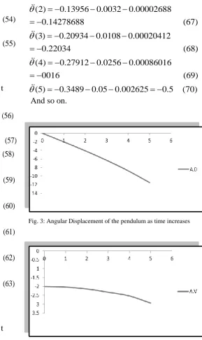
[image:5.595.301.556.574.705.2]Fig. 3: Angular Displacement of the pendulum as time increases
Fig. 4: Angular velocity of the pendulum as time increases
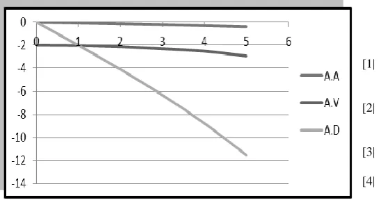
Fig. 6: Comparison of the angular Displacement, Velocity and Acceleration of the pendulum as time increases.
V. RESULT DISCUSSION AND CONCLUSION
In this study, firstly, equation of motion of inverted pendulum was formulated using Lagrangian equation, which involves both the kinetic and potential energies of the pendulum. Then differential transform method (DTM), as a semi analytical method, was adopted to analyse the resulted second order ordinary differential equation. With the assumptions and consideration of initial conditions, the solutions obtained were very close the ones obtained when solved analytically. From Figure 1 above, it can be seen that the angular displacement increases absolutely as time increases. This is always the case especially at the initial stage. Also the angular velocity and angular acceleration in figures 2 and figure 3 respectively increase with time, but at a lower rate when compared to the rate of angular displacement. This implies that the rate of change of angular displacement and the rate of change of velocity are mild compared to change in displacement itself. A closer look at figures 2 and figure 3 shows that the angular velocity at time t = 0, is -2, while the angular acceleration is 0. In figure 4, the comparison of the dynamic effect of the pendulum over a period of time, shows that angular displacement is more pronounced than the angular velocity. The angular acceleration is less than angular velocity. The negative values of the displacement, velocity, and acceleration as time increases resulted from the fact that the pendulum under consideration is an inverted pendulum. These results are in agreement with the ones in literature. DTM is very easy to use and reduces computation time.
REFERENCES
[1| What is an inverted pendulum?
https://wwrichard.net/2013/01/15/what-is-an inverted-pendulum/
[2| Filip Jeremi, Drivation of equation of motion for inverted pendulum problem, McMaster University, November 28, 2012
[3| Inverted pendulum from Wikipedia, the free Encyclopaedia https://en.wikipedia.org/wiki/Inverted_pendul
[4| M.C.Agarana and M.E. Emetere, (2016), Solving non-linear damped driven simple pendulum with small amplitude using a semi analytical method, ARPN Journal of Engineering and Applied Sciences, Vol 11, No 7, 2016
[5| M.C.Agarana and Agboola,2015,Dynamic Analysis of Damped driven pendulum using Laplace transform method, 26(3, 98-109)
[6| Biazar and M. Eslami, 2010. Differential transform Method for Quadratic Riccati Differential Equations. International Journal of Nonlinear Science. 9(4); 444 – 447
[7| M.C Agarana and S.A Iyase, 2015, Analysis of Hermite’s Equation Governing the motion of Damped Pendulum with small displacement, International Journal of Physical Sciences,10(2), 364 – 370
[8| Agarana M.C..and Bishop S.A, 2015, Quantitative Analysis of Equilibrium Solution and Stability for Non-linear Differential Equation Governing Pendulum Clock, International Journal of Applied Engineering Research, Vol. 10 No.24, pp.44112-44117
[9| Lagrangian mechanics. From Wikipedia, the Free encyclopaedia https://en.wikipedia.org/ wiki/Lagrangian_mechanic
[10] Haldun Alpaslan Peker, Onur Karaoğlu and Galip Oturanç, The Differential Transformation Method And Pade Approximant For A Form Of Blasius Equation, Mathematical and Computational Applications, Vol. 16, No. 2, pp. 507-513, 2011.