A. Artificial Neural Networks



Abstract— The prediction of a stock market price has been influenced by a set of the highly nonlinear financial and non-financial indicators may serve as a warning system for investors. In this research, the predicting of the future close price of Dow Jones Index Stocks was conducted using artificial neural networks. Feed forward neural network was used to predict next day closing in Dow Jones stock market. Nonlinear Autoregressive Exogenous (NARX) model is implemented by using feed forward neural network. To optimize the stock market price prediction, the performance of NARX model was examined and compared with different training algorithms. Although these algorithms had adequate results in predicting the NARX model with training, validation and testing. The Bayesian regularization has had the best performance in testing compared with levenberg-marquardt algorithm and the scaled conjugate gradient algorithm. While, the levenberg-marquardt algorithm has had less epochs in the best training performance of the network than the other algorithms. The performance of this model is found as a dominant model for stock market prediction.

Index Terms— Feed Forward Neural Network, Neural Networks, Nonlinear Autoregressive Exogenous, Stock Market Price.

I. INTRODUCTION

TOCK market price prediction is a very complex and challenging research area where different methods have been developed to predict stock price movement in the market [1]. Recently, artificial neural networks have been used as an auxiliary tool to predict stock price time series [2]. The novelties of neural networks lie in their ability to model nonlinear relations without a priori assumptions [3]. Neural networks have been useful to predict volatile financial variables, which are quite difficult to guess with classical statistical and econometric methods such as exchange rate and stock market [4]. Feed-forward neural networks are widely and successfully used models for classification, forecasting and problem solving [5]. Artificial neural network is a field of research which has enjoyed a rapid expansion in the literature for their ability to model nonlinear and multivariate processes without priori assumptions [3]. However, little attention has been paid to predict stock market price using neural-based nonlinear autoregressive exogenous model. Further, most research has been used stock pattern recognition model by matching template with many fixed weights assigned by researchers [6].

Thus, the aim of this research is to predict the future close price of the stock using promising classes of autoregressive network model. Dow Jones Index data set is used in this Qeethara K. Al-Shayea is with Department of Management Information Systems – Al Zaytoonah University of Jordan. Amman-Jordan, P. O Box 130 Amman 11733 (e-mail: [email protected]).

study because it represents 30 of the largest companies in the United States. The importance of Dow Jones comes from that the fluctuations of Dow Jones have some anticipating effect on other markets like German one [7]. Dow Jones Index stock is used as a data set to evaluate the performance of the proposed neural network. We use three algorithms (Levenberg-Marquardt algorithm, Bayesian Regularization, and the scaled conjugate gradient algorithm) with NARX model that allows predicting the future close price of the stock. From the results, it seems that using these algorithms are improved the accuracy of the model after each training stage. We show that the application of the NARX model enhances the performance of the proposed neural network methodology and improves the ability of it to predict the stock market price.

The rest of the paper is structured as follows. In section 2, we present the literature review and the architecture for the neural networks and NARX model. Section 3 describes the data and methodology used in this paper and the results of the empirical analysis. Finally, section 4 concludes the paper.

II. LITERATURE REVIEW

A. Artificial Neural Networks

In the last decades, many researchers have attempted to develop and enhance artificial neural networks methods to support the prediction in stock market segments. Cavalcante et. al. [8] presented a review of the recent computational intelligence approaches designed to solve financial market problems. The paper was focused on a specific financial market application or on machine learning algorithms fields. Mizuno et. al. [9] suggested a neural network model for technical analysis of stock market, and its application to a buying and selling timing prediction system for stock index. In their paper, a learning method is proposed for improving prediction accuracy of other categories, controlling the numbers of learning samples by using information about the importance of each category. Diaconescu [10] proved that an architectural approach of RNN with embedded memory, “Nonlinear Autoregressive model process with exogenous input” (NARX), showing promising qualities for dynamic system applications. He noticed that the performances of the NARX model are verified for several types of chaotic or fractal time series applied as input for neural network, in relation with the number of neurons, the training algorithms and the dimensions of his embedded memory. Wang [11] adopted artificial neural network (ANN) and two varieties of time series neural network to forecast the stock index of Chinese market. He mentioned that the NARX will be improved when more external data imported. A combination

Neural Networks to Predict Stock Market Price

Qeethara K. Al-Shayea, Member, IAENG

of data pre-processing methods involves genetic algorithm and Levenberg–Marquardt algorithm for learning feed forward neural networks for stock market prediction was proposed by Asadi et. al. [12]. Laboissierea, Fernandesb and Lage [13] was proposed an artificial neural network to forecasts the range of closing prices of three Brazilian power distribution companies’ stocks. Araújo [14] and Araújo [15] submitted two studies for Brazilian stock market prediction. Oztekin, Kizilaslan, Freund, and Iseri [16] was developed a methodology involving three models to predict daily stock price movements. These models are adaptive neuro-fuzzy inference systems, artificial neural net- works, and support vector machines. Zahedi and Rounaghi [17] assessed stock market prediction using artificial neural networks in Tehran Stock Exchange. Ou and Wang [18] applied ten data mining techniques to predict price movement of Hang Seng index of Hong Kong stock market. The approaches include Linear discriminant analysis (LDA), Quadratic discriminant analysis (QDA), K-nearest neighbor classification, Naïve Bayes based on kernel estimation, Logit model, Tree based classification, neural network, Bayesian classification with Gaussian process, Support vector machine (SVM) and Least squares support vector machine (SVM). Results showed that the SVM and LS-SVM generated superior predictive performance than the other models. Patel et. al. [19] presented four prediction models to predict the direction of movement of stock and stock price index for Indian stock markets. These models are Artificial Neural Network (ANN), Support Vector Machine (SVM), random forest and naive-Bayes with two approaches for input to these models. Experimental results with continuous-valued data shows that naive-Bayes (Gaussian process) model exhibits least performance while random forest exhibits highest performance. Oliveira, Nobre, and Zárate [20] proposed a neural network model for predictions of stocks closing prices future behaviour negotiated in BM&FBOVESPA in the short term, using the economic and financial theory, combining technical analysis, fundamental analysis and analysis of time series, to predict price behaviour, addressing the percentage of correct predictions of price series direction (POCID or Prediction of Change in Direction). As a case study, they used Petrobras stock PETR4, traded in BM&FBOVESPA. Experimental results show that he best performance was achieved with a window size of 3, which the POCID index of correct direction predictions was 93.62% for the test set and 87.50% for a validation set. Göçkena et. al. [21] presented a hybrid model based on a heuristic optimization methodology and artificial neural network to improve stock market forecasting performance in terms of statistical and financial terms. They applied the new model to predict stock price on Turkish stock market. They found that this model is a dominant model for stock market forecasting. Chiang et. al. [22] proposed an adaptive intelligent stock trading decision support system that utilizes particle swarm optimization and an artificial neural network to predict a stock index’s future movement direction. Hafezia, Shahrabib, and Hadavandi [23] presented bat-neural network multi-agent system as an intelligent model. After test the model to predict DAX stock price, results show that

the proposed model works better than other models. Bisoi & Dash [24] proposed a simple IIR filter based dynamic neural network and an innovative optimized adaptive unscented Kalman filter for forecasting stock price indices of four different Indian stocks. Four different learning strategies were used to adjust the weights of the dynamic neural information system. These strategies include gradient calculation, unscented Kalman filter (UKF), differential evolution (DE), and a hybrid technique (DEUKF) by alternately executing the DE and UKF for a few generations. Experimental results show that significant accuracy is achieved using the hybrid DEUKF algorithm than the others that include only DE, UKF, and gradient descent technique in chronological order. Qiu, Song, and Akagi [25] applied artificial neural network for the prediction of Japanese stock market. This paper presents nonlinear autoregressive exogenous models for future close price of Dow Jones stock index prediction. The proposed model used three different training algorithms which are called Levenberg-Marquardt algorithm, Bayesian regularization and Scaled conjugate gradient algorithm. According to the performance of this model, the three different training algorithms based neural network model is found as a dominant model for stock market prediction.

B. Neural Networks Architectures

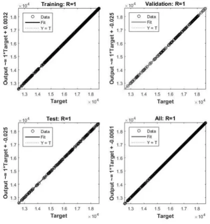
An ANN is a computational model that attempts to account for the parallel nature of the human brain. An ANN is a network of highly interconnecting processing elements (neurons) operating in parallel. Biological nervous systems inspire these elements. As in nature, the connections between elements largely determine the network function. A subgroup of processing element is called a layer in the network. The first layer is the input layer and the last layer is the output layer. Between the input and output layer, there may be additional layer(s) of units, called hidden layer(s). Fig. 1 represents the typical neural network. You can train a neural network to perform a function by adjusting the values of the connections (weights) between elements [5].

Fig. 1. A typical neural network.

The defining equation for the NARX model is

(1)

where the next value of the dependent output signal y(t) is regressed on previous values of the output signal and previous values of an independent (exogenous) input signal. You can implement the NARX model by using a feedforward neural network to approximate the function f. A diagram of the resulting network is shown below, where a two-layer feedforward network is used for the approximation. This implementation also allows for a vector ARX model, where the input and output can be multidimensional [26]. Fig. 2 illustrates the NARX model.

Fig. 2. The NARX Model.

There are many applications for the NARX network. It can be used as a predictor, to predict the next value of the input signal. It can also be used for nonlinear filtering, in which the target output is a noise-free version of the input signal. The use of the NARX network is shown in another important application, the modeling of nonlinear dynamic systems [26].

Some important qualities about NARX networks with gradient-descending learning gradient algorithm have been reported: (1) learning is more effective in NARX networks than in other neural network (the gradient descent is better in NARX) and (2) these networks converge much faster and generalize better than other networks [10] [27] [28].

Fig. 3 illustrate the proposed NARX model presented in this paper to predict the next day close price in Dow Jones Index stock.

Fig. 3. The proposed NARX.

Marquardt [29] indicated that the Levenberg-Marquardt (LM) algorithm is least-squares estimation of nonlinear parameters. It has been used to upgrade artificial neural

network weights [17]. The

Levenberg-Marquardt algorithm was designed to approach second-order training speed without having to compute the Hessian matrix. When the performance function has the form of a sum of squares (as is typical in training feedforward networks), then the Hessian matrix can be approximated as:

(2)

and the gradient can be computed as:

(3)

where is the Jacobian matrix that contains first derivatives of the network errors with respect to the weights and biases, and e is a vector of network errors. The Jacobian matrix can be computed through a standard backpropagation technique that is much less complex than computing the Hessian matrix.

The Levenberg-Marquardt algorithm uses this approximation to the Hessian matrix in the following Newton-like update:

(4)

When the scalar µ is zero, this is just Newton's method, using the approximate Hessian matrix. When µ is large, this becomes gradient descent with a small step size. Newton's method is faster and more accurate near an error minimum, so the aim is to shift toward Newton's method as quickly as possible. Thus, µ is decreased after each successful step (reduction in performance function) and is increased only when a tentative step would increase the performance function. In this way, the performance function is always reduced at each iteration of the algorithm.

This algorithm appears to be the fastest method for training moderate-sized feedforward neural networks (up to several hundred weights). It also has an efficient implementation in MATLAB® software, because the solution of the matrix equation is a built-in function, so its attributes become even more pronounced in a MATLAB environment [26].

Hagan and Menhaj [30] found after tested that the Marquardt algorithm on several function approximation problems is much more efficient than conjugate gradient algorithm and a variable learning rate algorithm when the network contains no more than a few hundred weights. Wilamowski [31] and Hagan & Menhaj [30] revealed that the LM optimization technique is more powerful than the conventional gradient descent techniques.

The scaled conjugate gradient algorithm is a supervised algorithm with feed forward backpropagation neural network. The scaled conjugate gradient algorithm (SCG), developed by Moller [32] was designed to avoid the time-consuming line search. This algorithm combines the model-trust region approach (used in the Levenberg-Marquardt algorithm described above in this study), with the conjugate gradient approach.

III. METHODOLOGY

A. Data Selection and Normalization

The data are obtained from the Yahoo/ finance website. It is daily data for Dow Jones Index stock. The parameters used as an indicator are the price of the stock at the beginning of the day (open), the highest price of the stock during the day (high), the lowest price of the stock during the day (low), the price of the stock at the end of the day (close) and the number of shares of stock that traded hands in the same day (volume). The closing price of the stock in the following day is used as output. At the same time, another financial indicator is used in this study, but it is found that there is no change in predicted next day close value. The dataset covers the time from January 2010 up to September 2016. The dataset is 1679 records. 1000 records are used in training the network while 679 records are used in testing the network.

B. Results and Performance Evaluation

A two-layer feed forward neural network with sigmoid hidden neurons and linear output neurons was created using dynamic time series neural network toolbox from MATLAB R2015a as shown in Fig 1. The network was trained and simulated with three algorithms.

The first algorithm implemented is Levenberg-Marquardt algorithm. The dataset used to train the network is 1000 sample while 679 sample is used to test the network. Fig. 4 shows the proposed network performance of the L-M algorithm. The best validation performance is equal to 0.0010071 at epoch 1000 and the training is stopped after 1000 epochs. Fig. 5 shows the training state value.

Fig. 4. The proposed network performance for L-M algorithm.

Fig. 5. The training state value.

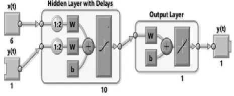
Fig. 6 shows regression plots display the network outputs with respect to targets for training, validation, and test sets. For a perfect fit, the data should fall along a 45-degree line, where the network outputs are equal to the targets. For this problem, the fit is reasonably good for all data sets, with R values in each case of 1. Fig. 7 illustrates the time series response which is displayed the inputs, targets, and errors versus time. It also indicates which time points were selected for training, testing and validation.

In Bayesian Regularization algorithm, the proposed network performance is shown in Fig. 8 while Fig. 9 shows the training state value. The best validation performance is equal to 0.44312 at epoch 1000 and the training is stopped after 1000 epochs. The dataset used to train the network is 1000 sample while 679 sample is used to test the network.

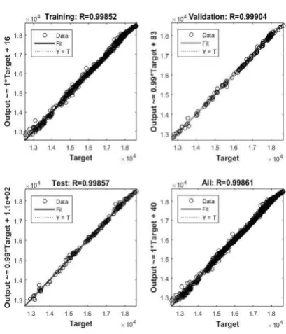
Fig. 10 shows regression plots display the network outputs with respect to targets for training, validation, and test sets. For a perfect fit, the data should fall along a 45-degree line, where the network outputs are equal to the targets. For this problem, the fit is reasonably good for all data sets, with R values in each case of 1. The time series response is illustrated in Fig. 11 which is displayed the inputs, targets and errors versus time. It also indicates which time points were selected for training, testing and validation

With SCG algorithm, the proposed network performance is shown in Fig. 12 while Fig. 13 shows the training state value. The best validation performance is equal to 4719.0433 at epoch 23 and the training is stopped after 29 epochs. The dataset used to train the network is 1000 sample while 679 sample is used to test the network.

Fig. 6. The regression plots.

Fig. 7. The time series response.

Fig. 8. The proposed network performance for Bayesian regularization.

Fig. 9. The training state value.

.

Fig. 10. The regression plots.

Fig. 12. The proposed network performance for SCG algorithm.

Fig. 13. The training state value.

Fig. 14. The regression plots.

Fig. 15. The time series response.

Table 1 shows the results after training the network while table 2 shows the results after simulating the network with the three algorithms we used it in the proposed model.

Table 1. Results after training the network Algorithm Phase MSE (Mean

Square Error)

R (Regression)

L-M ALGORITHM

Training 8.45569e-5 9.99999e-1

Validation 1.41385e-4 9.99999e-1

Testing 2.94345e-4 9.99999e-1

Bayesian regularization algorithm

Training 4.43115e-1 9.99999e-1

Testing 4.56249e-1 9.99999e-1

SCG ALGORITHM

Training 6649.78824e-0 9.98516e-1

Validation 4719.04325e-0 9.99040e-1

Testing 6052.19057e-0 9.98571e-1

Table 2. Results after testing the network

MSE (Mean Square Error) R (Regression)

L-M algorithm 71.99126e-0 9.99993e-1

Bayesian regularization

algorithm

249.86358e-0 9.99997e-1

SCG algorithm 1049125.49139e-0 9.37816e-1

IV. CONCLUSION

predicting stock price indices of the Dow Jones stock between January 2010 to September 2016. The advantage of NARX model is fast training and learning abilities and a high degree of prediction results. The results show that the proposed neural network model is coping with the fluctuation of the Dow Jones stock market prices and yields good predictive performance.

REFERENCES

[1] R. Rosas-Romero, A. Diaz-Torres, G. Etcheverry, “Forecasting of stock return prices with sparse representation of financial time series over redundant dictionaries”, Expert Systems with Applications, vol. 57, 2016, pp. 37-48.

[2] J. Wang & J. Wang, “Forecasting energy market indices with recurrent neural networks: Case study of crude oil price fluctuations”, Energy, vol. 102, 2016, pp. 365-374.

[3] H. Mo, J. Wang & H. Niu, “Exponent back propagation neural network forecasting for financial cross-correlation relationship”, Expert Systems with Applications, vol. 53, 2016, pp. 106–116. [4] A. D. Aydina & S. C. Cavdara, “Comparison of Prediction

Performances of Artificial Neural Network (ANN) and Vector Autoregressive (VAR) Models by Using the Macroeconomic Variables of Gold Prices”, Borsa Istanbul (BIST) 100 Index and US Dollar-Turkish Lira (USD/TRY) Exchange Rates, Procedia Economics and Finance, vol. 30, 2015, pp. 3-14.

[5] Q. Al-Shayea, G. El-Refae & S. Yaseen, “Artificial neural networks for medical diagnosis using biomedical dataset”, Int. J. Behavioural and Healthcare Research, vol. 4, no. 1, 2013, pp. 45-63.

[6] T. Chen & F. Chen, “An intelligent pattern recognition model for supporting investment decisions in stock market”, Information Sciences, vol. 346, 2016, pp. 261–274.

[7] A. Tangian, “Predicting DAX trends from Dow Jones data by methods of the mathematical theory of democracy”, European Journal of Operational Research, vol. 185, 2008, pp. 1632–1662.

[8] R. C. Cavalcante, R. C. Brasileiro, V. L. F. Souza, J. P. Nobrega & A. L. I. Oliveira, “Computational Intelligence and Financial Markets: A Survey and Future Directions”, Expert Systems with Applications, vol. 55, 2016, pp. 194-211.

[9] H. Mizuno, M. Kosaka, H. Yajima and N. Komoda, “Application of Neural Network to Technical Analysis of Stock Market Prediction”, Studies in Informatics, and Control, vol. 7, no. 3, 1998, pp. 111–120. [10] E. Diaconescu, “The use of NARX neural networks to predict chaotic

time series”, WSEAS Transactions on Computer Research, vol. 3, 2008, pp. 182-191.

[11] C. Wang, “Time series neural network systems in stock index forecasting”, Computer Modelling & New Technologies, 19(1B), 2015, pp. 57-61.

[12] S. Asadi, E. Hadavandi, F. Mehmanpazir & M. Nakhostin, “Hybridization of evolutionary Levenberg–Marquardt neural networks and data”, Knowledge-based system, vol. 35, 2012, pp. 245-258.

[13] L. A. Laboissierea, R. A. S. Fernandesb and G. G. Lage, “Maximum and minimum stock price forecasting of Brazilian power distribution companies based on artificial neural networks”, Applied soft computing, vol. 35, 2015, pp. 66-74.

[14] R. A. Araújo, “Hybrid intelligent methodology to design translation invariant morphological operators for Brazilian stock market prediction”, Neural Networks, vol. 23, 2010, pp. 1238-1251. [15] R. A. Araújo, “A morphological perceptron with gradient-based

learning for Brazilian stock market forecasting”, Neural Networks, vol. 28, 2012, pp. 61-81.

[16] A. Oztekin, R. Kizilaslan, S. Freund & A. Iseri, “A data analytic approach to forecasting daily stock returns in an emerging market”, European Journal of Operational Research, vol. 253, 2016, pp. 697-710.

[17] J. Zahedi & M. Rounaghi, “Application of artificial neural network models and principal component analysis method in predicting stock prices on Tehran Stock Exchange”, Physica A, vol. 438, 2015, pp. 178-187.

[18] P. Ou & H. Wang, “Prediction of stock market index movement by ten data mining techniques”, Modern Applied Science, vol. 3, P28, 2009.

[19] J. Patel, S. Shah, P. Thakkar & K. Kotecha, “Predicting stock and stock price index movement using Trend Deterministic Data Preparation and machine learning techniques,” Expert Systems with Applications, vol. 42, 2015, pp. 259-268.

[20] F. A. Oliveira, C. N. Nobre & L. E. Zárate, “Applying Artificial Neural Networks to prediction of stock price and improvement of the directional prediction index – Case study of PETR4”, Petrobras, Brazil, Expert Systems with Applications, vol. 40, 2013, pp. 7596-7606.

[21] M. Göçkena, M. Özçalıcıb, A. Borua & A. T. Dosdogruc, “Integrating metaheuristics and Artificial Neural Networks for improved stock price prediction”, Expert Systems with Applications, vol. 44, 2016, pp. 320-331.

[22] W. Chiang, D. Enke, T. Wu & R. Wang, “An adaptive stock index trading decision support system”, Expert Systems with Applications, vol. 59, 2016, pp. 195-207.

[23] R. Hafezia, J. Shahrabib & E. Hadavandi, “A bat-neural network multi-agent system (BNNMAS) for stock price prediction: Case study of DAX stock price”, Applied Soft Computing, vol. 29, 2015, pp. 196-210.

[24] R. Bisoi & P. K. Dash, “A hybrid evolutionary dynamic neural network for stock market trend analysis and prediction using unscented Kalman filter”, Applied Soft Computing, vol. 19, 2014, pp. 41-56.

[25] M. Qiu, Y. Song & F. Akagi, “Application of artificial neural network for the prediction of stock market returns: The case of the Japanese stock market”, Chaos, Solitons & Fractals, 2016, pp. 85, 1–7. [26] M. H. Beale, M. T. Hagan and H. B. Demuth, Neural Network

Toolbox User’s Guide. The MathWorks Inc., 2015.

[27] T. Lin, B. G. Horne, P. Tino & C. L. Giles, “Learning long-term dependencies in NARX recurrent neural networks”, IEEE Transactions on Neural Networks, vol. 7, no. 6, 1996, pp. 1329-1351. [28] Y. Gao and M. J. Er, “NARMAX time series model prediction: feedforward and recurrent fuzzy neural network approaches”, Fuzzy Sets and Systems, vol. 150, no. 2, 2005, pp. 331-350.

[29] D. W. Marquardt, “An Algorithm for the Least-Squares Estimation of Nonlinear Parameters”, SIAM Journal of Applied Mathematics, vol. 11, no. 2, 1963, pp. 431–441.

[30] M. T. Hagan and M. Menhaj, “Training feed-forward networks with the Marquardt algorithm”, IEEE Transactions on Neural Networks, vol. 5, no. 6, 1994, pp. 989–993.

[31] B. M. Wilamowski, “Neural network architectures and learning algorithms”, Industrial Electronics Magazine IEEE, vol. 3, no. 4, 2009, pp. 56-63.

[32] M. F. Moller, “A scaled conjugate gradient algorithm for fast supervised learning”, Neural Networks, vol. 6, 1993, pp. 525–533.

Assoc. Prof. Dr. Qeethara Kadhim Abdulrahman Al-Shayea has