Abstract— In this paper, the differential calculus was used to obtain some classes of ordinary differential equations (ODE) for the probability density function, quantile function, survival function, inverse survival function, hazard function and reversed hazard function of the Frĕchet distribution. The stated necessary conditions required for the existence of the ODEs are consistent with the various parameters that defined the distribution. Solutions of these ODEs by using numerous available methods are a new ways of understanding the nature of the probability functions that characterize the distribution. The method can be extended to other probability distributions and can serve an alternative to approximation.
Index Terms— Quantile function, Frĕchet distribution, reversed hazard function, calculus, differentiation, probability density function.
I. INTRODUCTION
RȆCHET distribution is one of the mostly applied distributions in extreme value theory. Detailed information about the distribution can be obtained from the early works of [1] and [2] and book written by [3]. Different methods of estimation of the parameters of the distribution were discussed extensively by [4]. Some of the applications are as follows: Zaharim et al. [5] used the distribution to model wind speed data, Harlow [6] worked on the usefulness of the distribution in modeling engineering problems, Nadarajah and Kotz [7] discussed extensively on the application of the Fréchet random variables to sociological models. Vovoras and Tsokos [8] used the distribution to model and analyze precipitation data. Details on the application of the distribution in modeling extremal data can be found in [9]. Many authors and researchers have proposed modifications or developed generalizations of the distribution. Some of them are: beta Fréchet distribution [10] [11], Kumaraswamy Fréchet distribution [12], transmuted Fréchet distribution [13], transmuted exponentiated Fréchet distribution [14], gamma extended Fréchet distribution [15], Marshall–Olkin Fréchet distribution [16], transmuted Marshall–Olkin Fréchet
This work was sponsored by Covenant University, Ota, Nigeria. H. I. Okagbue, P. E. Oguntunde, A. A. Opanuga and E. A. Owoloko are with the Department of Mathematics, Covenant University, Ota, Nigeria.
[email protected] [email protected] [email protected] [email protected]
distribution [17], Weibull Fréchet distribution [18], six-parameter Fréchet distribution [19], beta exponential Fréchet distribution [20]
The aim of this research is to develop ordinary differential equations (ODE) for the probability density function (PDF), Quantile function (QF), survival function (SF), inverse survival function (ISF), hazard function (HF) and reversed hazard function (RHF) of Fréchet distribution by the use of differential calculus. Calculus is a very key tool in the determination of mode of a given probability distribution and in estimation of parameters of probability distributions, amongst other uses. The research is an extension of the ODE to other probability functions other than the PDF. Similar works done where the PDF of probability distributions was expressed as ODE whose solution is the PDF are available. They include: Laplace distribution [21], beta distribution [22], raised cosine distribution [23], Lomax distribution [24], beta prime distribution or inverted beta distribution [25].
II. PROBABILITY DENSITY FUNCTION
The probability density function of the Frȇchet distribution is given as;
( 1)
( )
e
xf x
x
(1)To obtain the first order ordinary differential equation for the probability density function of the Frȇchet distribution, differentiate equation (1), to obtain;
1
( 2) 2
( 1)
e
(
1)
( )
( )
e
x
x
x
x
x
f x
f x
x
(2)
1 2
(
1)
( )
( )
f x
f x
x
x
x
(3)The condition necessary for the existence of equation is
, ,
x
0.
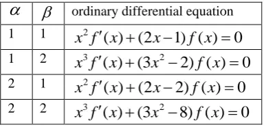
The first order ordinary differential equations can beobtained for the particular values of the parameters. The few cases are summarized in the Table 1.
Classes of Ordinary Differential Equations
Obtained for the Probability Functions of
Frĕchet Distribution
Hilary I. Okagbue, Member, IAENG, Pelumi E. Oguntunde, Abiodun A. Opanuga,
Enahoro A. Owoloko
Table 1: Classes of differential equations obtained for the probability density function of the Frȇchet distribution for different parameters.
ordinary differential equation1 1 2
( ) (2
1) ( )
0
x f x
x
f x
1 2 3 2
( ) (3
2) ( )
0
x f x
x
f x
2 1 2
( ) (2
2) ( )
0
x f x
x
f x
2 2 3 2
( ) (3
8) ( )
0
x f x
x
f x
Equation (3) is differentiated in an attempt to obtain ordinary differential equations that are not dependent on the powers of the parameters.
2 2
2 4
1 3
1 2
(
1)
(
1)
( )
( )
2
(
1)
+
( )
x
x
x
f
x
f x
x
x
f x
x
x
x
(4) The condition necessary for the existence of equation (4) is
, ,
x
0.
The following equations obtained from equation (3) are needed in the simplification of equation (4);1 2
( )
(
1)
( )
f x
f x
x
x
x
(5)
1 2
( )
1
( )
f x
x
x
f x
x
(6)
1 2
2
( )
1
2
( )
f x
x
x
f x
x
(7)
1 3
2
2
( )
1
( )
f x
x
x
x
f x
x
(8)1 2
2
(
1)
( )
1
(
1)
( )
f x
x
x
f x
x
(9)1 2
4 2
(
1)
(
1)
( )
1
( )
f x
x
x
x
f x
x
(10)
2 2
4
(
1)
1
( )
1
( )
f x
x
x
x
f x
x
(11)Substitute equations (5), (8) and (11) into equation (4) to obtain;
2 2
( 1) 1 ( ) 1
( ) ( )
( ) ( )
( ) 2 ( ) 1
( )
f x
x x f x x
f x
f x f x
f x f x
x f x x
(12)
2
2
( )
(
1)
( )
(
1) ( )
( )
( )
f
x
f x
f x
f
x
f x
x
x
(13)The second order ordinary differential equation for the probability density function of the Frȇchet distribution is given by;
2 2 2
2
( )
( )
( )
(
1)
( )
( )
(
1)
( )
0
x f x f
x
x f
x
xf x f x
f
x
(14)(1)
e
f
(15)
(1)
(
1)
e
f
(16)III. QUANTILE FUNCTION
The Quantile function of the Frȇchet distribution is given as;
( )
11
ln
Q p
p
(17) To obtain the first order ordinary differential equation for the Quantile function of the Frȇchet distribution, differentiate equation (17), to obtain;
1 1
( )
1
ln
Q p
p
p
(18)
Substitute equation (17) into (18);
( )
( )
1
ln
Q p
Q p
p
p
(19)
The condition necessary for the existence of equation is
,
0, 0
p
1.
Equation (17) can also be written as;1
ln
( )
p
Q
p
(20) Substitute equation (20) into (19);1
( )
( )
( )
( )
Q p Q
p
Q
p
Q p
p
p
(21)1
( )
( )
0
p
Q p
Q
p
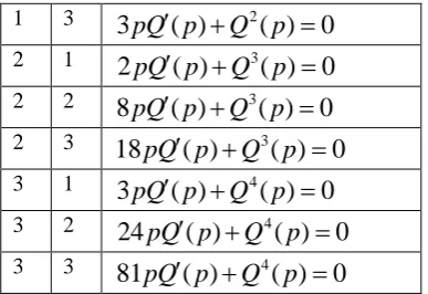
(22) The first order ordinary differential equations can be obtained for the particular values of the parameters obtained from equation (22). The few cases are summarized in Table 2.
Table 2: Classes of differential equations obtained for the quantile function of the Frȇchet distribution for different parameters.
ordinary differential equation 1 1pQ p
( )
Q p
2( )
0
1 2 2
[image:2.595.73.267.96.189.2] [image:2.595.57.278.238.359.2]1 3 2
3
pQ p
( )
Q p
( )
0
2 1 3
2
pQ p
( )
Q p
( )
0
2 2 3
8
pQ p
( )
Q p
( )
0
2 3 3
18
pQ p
( )
Q p
( )
0
3 1 4
3
pQ p
( )
Q p
( )
0
3 2 4
24
pQ p
( )
Q p
( )
0
3 3 4
81
pQ p
( )
Q p
( )
0
Equation (18) is differentiated in an attempt to obtain ordinary differential equations that are not dependent on the powers of the parameters.
1 ( 2)
2
1 ( 1)
1
1
1
ln
( )
( )
1
1
ln
p
p
p
Q p
Q p
p
p
(23) The condition necessary for the existence of equation is
,
0, 0
p
1.
1
1
( )
( )
1
ln
Q p
Q p
p
p
p
(24)
Equation (19) can also be written as;
( )
1
( )
1
ln
Q p
Q p
p
p
(25)
Substitute equation (25) into (24);
1
(1
)
( )
( )
( )
( )
Q p
Q p
Q p
p
Q p
(26)The second order ordinary differential equation for the Quantile function of the Frȇchet distribution is given by;
2
( )
( ) (1
)
( )
( )
( )
0
pQ p Q p
pQ
p
Q p Q p
(27)(0.1)
12.3026
Q
(28)1 1
10
(0.1)
(2.3026)
Q
(29)Some cases can be considered such as: When
1,
equations(27)-(29) become;2
( )
( ) 2
( )
( )
( )
0
pQ p Q p
pQ
p
Q p Q p
(30)(0.1)
2.3026
Q
(31)2
10
(0.1)
1.8860925
(2.3026)
Q
(32)IV. SURVIVAL FUNCTION
The survival function of the Frȇchet distribution is given as;
S t
( ) 1 e
t
(33) To obtain the first order ordinary differential equation for the survival function of the Frȇchet distribution, differentiate equation (33), to obtain;1 2
( )
e
tS t
t
t
(34)( 1)
( )
e
tS t
t
(35) The condition necessary for the existence of equation is, ,
t
0.
Equation (33) can also be written as;e
tS t
( ) 1
(36) Substitute equation (36) into equation (35);( 1)
( )
( ( ) 1)
S t
t
S t
(37) The first order ordinary differential equations can be obtained for the particular values of the parameters obtained from equation (37). The few cases are summarized in Table 3.Table 3: Classes of differential equations obtained for the survival function of the Frȇchet distribution for different parameters.
Ordinary differential equation1 1 2
( )
( ) 1 0
t S t
S t
1 2 2
( ) 2 ( ) 2
0
t S t
S t
1 3 2
( ) 3 ( ) 3
0
t S t
S t
2 1 3
( ) 2 ( ) 2
0
t S t
S t
2 2 3
( ) 8 ( ) 8
0
t S t
S t
2 3 3
( ) 18 ( ) 18
0
t S t
S t
3 1 4
( ) 3 ( ) 3
0
t S t
S t
3 2 4
( ) 24 ( ) 24
0
t S t
S t
3 3 4
( ) 81 ( ) 81 0
t S t
S t
[image:3.595.73.267.49.182.2]1 ( 2) 2
( 1)
e
(
1)
( )
( )
e
t
t
t
t
t
S t
S t
t
(38) The condition necessary for the existence of equation is
, ,
t
0.
1 2
(
1)
( )
( )
S t
S t
t
t
t
(39)1
(
1)
( )
( )
S t
S t
t
t
(40)Equation (37) can also be written as;
1
( )
( ) 1
S t
S t
t
(41) Substitute equation (41) into equation (40);
( )
( )
(
1)
( )
( ) 1
S t
S t
S t
S t
t
(42)The second order ordinary differential equation for the survival function of the Frȇchet distribution is given by;
2
( ( ) 1)
( )
( ) (
1)( ( ) 1) ( )
0
t S t
S t
tS
t
S t
S t
(43)S
(1) 1 e
(44)S
(1)
e
(45)Some cases can be considered such as: When
1,
equations(43)-(45) become;2
( ( ) 1)
( )
( ) 2( ( ) 1) ( )
0
t S t
S t
tS
t
S t
S t
(46)(1) 1 e
S
(47)(1)
e
S
(48)V. INVERSE SURVIVAL FUNCTION
The inverse survival function of the Frȇchet distribution is given as;
1
( )
1
ln
1
Q p
p
(49)
To obtain the first order ordinary differential equation for the inverse survival function of the Frȇchet distribution, differentiate equation (49), to obtain;
1 1
( )
1
(1
) ln
1
Q p
p
p
(50)
Substitute equation (49) into (50);
( )
( )
1
(1
) ln
1
Q p
Q p
p
p
(51)
The condition necessary for the existence of equation is
,
0, 0
p
1.
Equation (49) can also be written as;1
ln
1
p
Q
( )
p
(52) Substitute equation (52) into (51);1
( )
( )
( )
( )
(1
)
(1
)
Q p Q
p
Q
p
Q p
p
p
(53)1
(1
p Q p
)
( )
Q
( )
p
0
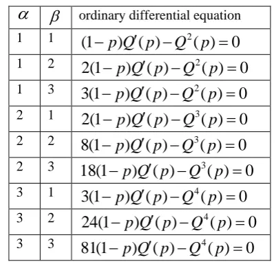
(54) The first order ordinary differential equations can be obtained for the particular values of the parameters obtained from equation (54). The few cases are summarized in Table 4.
Table 4: Classes of differential equations obtained for the inverse survival function of the Frȇchet distribution for different parameters .
ordinary differential equation1 1 2
(1
p Q p
)
( )
Q p
( )
0
1 2 2
2(1
p Q p
)
( )
Q p
( )
0
1 3 2
3(1
p Q p
)
( )
Q p
( )
0
2 1 3
2(1
p Q p
)
( )
Q p
( )
0
2 2 3
8(1
p Q p
)
( )
Q p
( )
0
2 3 3
18(1
p Q p
)
( )
Q p
( )
0
3 1 4
3(1
p Q p
)
( )
Q p
( )
0
3 2 4
24(1
p Q p
)
( )
Q p
( )
0
3 3 4
81(1
p Q p
)
( )
Q p
( )
0
VI. HAZARD FUNCTION
The hazard function of the Frȇchet distribution is given as;
( 1)
e
( )
1 e
t
t
t
h t
(55)
( 1)
( )
e
t1
t
h t
(56)
[image:4.595.325.526.420.612.2]( 2) ( 1)
1
2 2
1
(
1)
( )
e
(e
1)
( )
(e
1)
t t
t
t
t
h t
h t
t
t
(57)
The condition necessary for the existence of equation is
, ,
t
0.
( 1)
(
1)
e
( )
( )
(e
1)
t
t
t
h t
h t
t
(58)
(
1)
( )
( ) e
t( )
h t
h t
h t
t
(59)
Equation (56) can be simplified as;
( 1) ( 1)
( )
e
1
( )
( )
t
t
t
h t
h t
h t
(60) Substitute equation (60) into equation (59);
( 1)
(
1)
( )
( )
( )
h t
t
h t
h t
t
(61)2
( )
( ) (
(
1)) ( )
0
th t
h t
t
h t
(62) Differentiation is carried out again in order to obtain an ordinary differential equation that does not contain the powers of the parameters.;1
2 2
(
1)
( )
( ) e
( )
(
1)
( ) e
e
( )
( )
t
t t
h t
h t
h t
t
h t
h t
h t
t
t
t
(63) The condition necessary for the existence of equation is
, ,
t
0.
The following equations obtained from equation (59) are needed to simplify equation (63);( )
(
1)
( ) e
( )
t
h t
h t
h t
t
(64)
( ) e
( )
(
1)
( )
t
h t
h t
h t
t
(65)
e
( )
1
( )
t
h t
th t
(66) Substitute equations (64) and (66) into equation (63);
2
2
2 1
( )
(
1)
( )
( )
( )
1
( )
( ) ( )
( )
1
( )
( )
( )
h
t
h t
h t
h t
t
h t
h t h t
th t
h t
h t
t
th t
(67)
When
1,
equation (67) becomes;2
2
2 2
( )
2 ( )
( )
( )
2
( )
( ) ( )
( )
2
( )
( )
( )
h
t
h t
h t
h t
t
h t
h t h t
th t
h t
h t
t
th t
(68)
VII. REVERSED HAZARD FUNCTION
The reversed hazard function of the Frȇchet distribution is given as;
( 1)
( )
j t
t
(69)( 1)
( 2)
(
1)
( )
(
1)
t
j t
t
t
(70) The condition necessary for the existence of equation is
, ,
t
0.
Substitute equation (69) into equation (70) to obtain;
(
1)
( )
( )
j t
j t
t
(71) The first order ordinary differential equation for the reversed hazard function of the Frȇchet distribution is given by;tj t
( ) (
1) ( )
j t
0
(72)j
(1)
(73)The ODEs of all the probability functions considered can be obtained for the particular values of the distribution. Several analytic, semi-analytic and numerical methods can be applied to obtain the solutions of the respective differential equations [26-40]. Also comparison with two or more solution methods is useful in understanding the link between ODEs and the probability distributions.
VIII. CONCLUDING REMARKS
others. In all, the parameters that define the distribution determine the nature of the respective ODEs and the range determines the existence of the ODEs.
ACKNOWLEDGMENT
The authors are unanimous in appreciation of financial sponsorship from Covenant University. The constructive suggestions of the reviewers are greatly appreciated.
REFERENCES
[1] M. Fréchet, “Sur la Loi des Erreurs d’Observation”, Bulletin Société Mathé. Moscou, vol. 33, pp. 5-8, 1924.
[2] M. Fréchet, :Sur la loi de probabilité de l'écart maximum”, Ann. Soc. Polon. Math., vol. 6, pp. 93-122, 1928.
[3] S. Kotz and S. Nadarajah, Extreme Value Distributions: Theory and Applications, Imperial College Press, London. ISBN: 1860942245 9781860942242, 2002.
[4] A.N. Joshi and D.K. Ghosh, “Frechet distribution : Parametric estimation and its comparison by different methods of estimation”,
Int. J. Agric. Stat. Sci., vol. 12, no. 2, pp. 365-375, 2015.
[5] A. Zaharim, S.K. Najid, A.M. Razali and K. Sopian, “Analysing Malaysian wind speed data using statistical distribution”, Proc. WSEAS Int. Conf. Energy and Environ., Cambridge, 2009. [6] D.G. Harlow, “Applications of the Fréchet distribution function”, Int.
J. Mater. Prod. Technol. Vol. 17, pp. 482–495, 2002.
[7] S. Nadarajah and S. Kotz, “Sociological models based on Fréchet random variables”, Qual. Quant., vol. 42, pp. 89–95, 2008. [8] D. Vovoras and C.P. Tsokos, “Statistical analysis and modeling of
precipitation data”, Nonl. Anal. Theo. Meth. Appl., vol. 71, no. 12, pp. e1169-e1177, 2009.
[9] K. Müller and W.D. Richter, “Modelling extremal data”, J. Stat. Comput. Simul., vol. 87, no. 5, pp. 933-955, 2017.
[10] S. Nadarajah and A.K. Gupta, “The beta Fréchet distribution”, Far East J. Theor. Stat. vol. 14, pp. 15–24, 2004.
[11] W. Barreto-Souza, G.M. Cordeiro and A.B. Simas, “Some results for beta Fréchet distribution”, Comm. Stat. Theo. Meth., vol. 40, pp. 798– 811, 2011.
[12] M.E. Mead and A.R. Abd-Eltawab, “A note on Kumaraswamy Fréchet distribution”, Aust. J. Basic Appl. Sci. vol. 8, pp. 294–300, 2014.
[13] M.R. Mahmoud and R.M. Mandouh, “On the transmuted Fréchet distribution”, J. Appl. Sci. Res., vol. 9, pp. 5553–5561, 2013. [14] I. Elbatal, G. Asha and V. Raja, “Transmuted exponentiated Fréchet
distribution: Properties and applications”, J. Stat. Appl. Prob., vol. 3, pp. 379–394, 2014.
[15] R.V. da Silva, T.A.N. de Andrade, D.B.M. Maciel, R.P.S. Campos and G.M. Cordeiro, “A new lifetime model: The gamma extended Fréchet distribution”, J. Stat. Theo. Appl., vol. 12, pp. 39–54, 2013. [16] E. Krishna, K.K. Jose, T. Alice and M.M. Ristic, “The Marshall–
Olkin Fréchet distribution”, Comm. Stat. Theo. Meth., vol. 42, pp. 4091–4107, 2013.
[17] A.Z. Afify, G.G. Hamedani, I. Ghosh and M.E. Mead, “The transmuted Marshall–Olkin Fréchet distribution: Properties and applications”, Int. J. Stat. Prob., vol. 4, pp. 132–148, 2015. [18] A.Z. Afify, H.M. Yousof, G.M. Cordeiro, E.M.M. Ortega and Z.M.
Nofal, “The Weibull Fréchet distribution and its applications”, J. Appl. Stat., vol. 43, no. 14, pp. 2608-2626, 2016.
[19] H.M. Yousof, A.Z. Afify, A.E.H.N. Ebraheim, G.G. Hamedani and N.S. Butt, “On six-parameter fréchet distribution: Properties and applications”, Pak. J. Stat. Oper. Res., vol. 12, no. 2, pp. 281-299, 2016.
[20] M.E. Mead, A.Z. Afify, G.G. Hamedani and I. Ghosh, “The beta exponential Fréchet distribution with applications”, Austrian J. Stat.,
vol. 46, no. 1, pp. 41-63, 2017. [21] N.L. Johnson, S. Kotz and N. Balakrishnan, Continuous univariate
distributions, Wiley New York. ISBN: 0-471-58495-9, 1994. [22] W.P. Elderton, Frequency curves and correlation, Charles and Edwin
Layton. London, 1906.
[23] H. Rinne, Location scale distributions, linear estimation and probability plotting using MATLAB, 2010.
[24] N. Balakrishnan and C.D. Lai, Continuous bivariate distributions, 2nd edition, Springer New York, London, 2009.
[25] N.L. Johnson, S. Kotz and N. Balakrishnan, Continuous Univariate Distributions, Volume 2. 2nd edition, Wiley, 1995.
[26] S.O. Edeki, H.I. Okagbue , A.A. Opanuga and S.A. Adeosun, “A semi - analytical method for solutions of a certain class of second order ordinary differential equations”, Applied Mathematics, vol. 5, no. 13, pp. 2034 – 2041, 2014.
[27] S.O. Edeki, A.A Opanuga and H.I Okagbue, “On iterative techniques for numerical solutions of linear and nonlinear differential equations”,
J. Math. Computational Sci., vol. 4, no. 4, pp. 716-727, 2014. [28] A.A. Opanuga, S.O. Edeki, H.I. Okagbue, G.O. Akinlabi, A.S.
Osheku and B. Ajayi, “On numerical solutions of systems of ordinary differential equations by numerical-analytical method”, Appl. Math. Sciences, vol. 8, no. 164, pp. 8199 – 8207, 2014.
[29] S.O. Edeki , A.A. Opanuga, H.I. Okagbue , G.O. Akinlabi, S.A. Adeosun and A.S. Osheku, “A Numerical-computational technique for solving transformed Cauchy-Euler equidimensional equations of homogenous type. Adv. Studies Theo. Physics, vol. 9, no. 2, pp. 85 – 92, 2015.
[30] S.O. Edeki , E.A. Owoloko , A.S. Osheku , A.A. Opanuga , H.I. Okagbue and G.O. Akinlabi, “Numerical solutions of nonlinear biochemical model using a hybrid numerical-analytical technique”,
Int. J. Math. Analysis, vol. 9, no. 8, pp. 403-416, 2015.
[31] A.A. Opanuga , S.O. Edeki , H.I. Okagbue and G.O. Akinlabi, “Numerical solution of two-point boundary value problems via differential transform method”, Global J. Pure Appl. Math., vol. 11, no. 2, pp. 801-806, 2015.
[32] A.A. Opanuga, S.O. Edeki, H.I. Okagbue and G. O. Akinlabi, “A novel approach for solving quadratic Riccati differential equations”,
Int. J. Appl. Engine. Res., vol. 10, no. 11, pp. 29121-29126, 2015. [33] A.A Opanuga, O.O. Agboola and H.I. Okagbue, “Approximate
solution of multipoint boundary value problems”, J. Engine. Appl. Sci., vol. 10, no. 4, pp. 85-89, 2015.
[34] A.A. Opanuga, O.O. Agboola, H.I. Okagbue and J.G. Oghonyon, “Solution of differential equations by three semi-analytical techniques”, Int. J. Appl. Engine. Res., vol. 10, no. 18, pp. 39168-39174, 2015.
[35] A.A. Opanuga, H.I. Okagbue, S.O. Edeki and O.O. Agboola, “Differential transform technique for higher order boundary value problems”, Modern Appl. Sci., vol. 9, no. 13, pp. 224-230, 2015. [36] A.A. Opanuga, S.O. Edeki, H.I. Okagbue, S.A. Adeosun and M.E.
Adeosun, “Some Methods of Numerical Solutions of Singular System of Transistor Circuits”, J. Comp. Theo. Nanosci., vol. 12, no. 10, pp. 3285-3289, 2015.
[37] A.A. Opanuga, H.I. Okagbue, O.O. Agboola, "Irreversibility Analysis of a Radiative MHD Poiseuille Flow through Porous Medium with Slip Condition," Lecture Notes in Engineering and Computer Science: Proceedings of The World Congress on Engineering 2017, 5-7 July, 2017, London, U.K., pp. 167-171. [38] A.A. Opanuga, E.A. Owoloko, H.I. Okagbue, “Comparison
Homotopy Perturbation and Adomian Decomposition Techniques for Parabolic Equations,” Lecture Notes in Engineering and Computer Science: Proceedings of The World Congress on Engineering 2017, 5-7 July, 2017, London, U.K., pp. 24-27.
[39] A.A. Opanuga, E.A. Owoloko, H. I. Okagbue, O.O. Agboola, "Finite Difference Method and Laplace Transform for Boundary Value Problems," Lecture Notes in Engineering and Computer Science: Proceedings of The World Congress on Engineering 2017, 5-7 July, 2017, London, U.K., pp. 65-69.
[40] A.A. Opanuga, E.A. Owoloko, O.O. Agboola, H.I. Okagbue, "Application of Homotopy Perturbation and Modified Adomian Decomposition Methods for Higher Order Boundary Value Problems," Lecture Notes in Engineering and Computer Science: Proceedings of The World Congress on Engineering 2017, 5-7 July, 2017, London, U.K., pp. 130-134.