An Application of Fuzzy Inference System Composed of Double-Input Rule Modules to Control Problems

(1)

An Application of Fuzzy Inference System

Composed of Double-Input Rule Modules to

Control Problems

Hirofumi Miyajima

†1

, Fumihiro Kawai

†2

, Noritaka Shigei

†3

, and Hiromi Miyajima

†4

Abstract—The automatic construction of fuzzy system with a large number of input variables involves many difficulties such as large time complexity and getting stuck in a shallow and local minimum. As models to overcome them, the SIRMs (Single-Input Rule Modules) and DIRMs(Double-(Single-Input Rule Modules) models have been proposed. In some numerical simulations such as EX-OR problem, it was shown that there exists the difference of the ability between DIRMs and SIRMs models. In this paper, we will apply DIRMs and SIRMs models to control problem such as obstacle avoidance. As a result, it is shown that DIRMs model is also more effective than SIRMs model about control problem. Further, we propose a constructive DIRMs model with the reduced number of modules and show the effectiveness in numerical simulations.

Index Terms—Fuzzy inference model, Single-input rule mod-ule, Small number of input rule modmod-ule, Double input rule module, obstacle avoidance.

I. INTRODUCTION

M

ANY studies on self-tuning fuzzy systems[1], [2] have been made. The aim of these studies is to construct automatically fuzzy reasoning rules from input and output data based on the steepest descend method. Obvious drawbacks of the steepest descend method are its large com-putational complexity and getting stuck in a shallow local minimum. In order to overcome them, some novel methods have been developed as shown in the references[3], [4], [5], [6], [7]. The SIRMs (Single-Input Rule Modules) model aims to obtain a better solution by using fuzzy inference system composed of SIRMs[8], where output is determined as the weighted sum of all modules. However, it is known that the SIRMs model does not always achieve good performance in non-linear problems. Therefore, we have proposed the SNIRMs (Small Number of Input Rule Modules) model as a generalized SIRMs model, in which each module is composed of small number of input variables[9]. DIRMs (Double-Input Rule Modules) model is an example of such models and each module of DIRMs model is composed of two input variables. It is well known that EX-OR problem with two input variables can be approximated by DIRMs model but not by SIRMs model[10]. Further, there exists the difference of the ability between DIRMs and SIRMs models as shown later in the paper. Then, does there exist such example in control problems? In this paper, we consider the

Affiliation: Graduate School of Science and Engineering, Kagoshima University, 1-21-40 Korimoto, Kagoshima 890-0065, Japan

corresponding author to provide email: miya@eee.kagoshima-u-ac.jp

†1email: k3768085@kadai.jp †2email: k8005442@kadai.jp †3email: shigei@eee.kagoshima-u-ac.jp †4email: miya@eee.kagoshima-u-ac.jp

obstacle avoidance problem as an example of such problems. The problem is how does the agent (or robot) avoid the obstacle and reach the specified point. We show that DIRMs model can simulate the problem but SIRMs model can not. The simulation results show that the proposed methods are also superior in control problem to the conventional SIRMs model.

II. FUZZYINFERENCEMODEL AND ITSLEARNING

A. Fuzzy Inference Model

The conventional fuzzy inference model using the steepest descend method is described[1]. LetZj={1,· · ·, j}for the positive integerj. Letx= (x1,· · ·, xm)andy be input and output data, respectively, wherexifori∈Zmandyare real number. Then the rule of simplified fuzzy inference model is expressed as

Rj : if x1 isM1j and · · · andxm isMmj theny iswj,

(1) wherej∈Znis a rule number,i∈ Zmis a variable number,

Mij is a membership function of the antecedent part, andwj is the weight of the consequent part.

A membership value of the antecedent partµifor inputx is expressed as

µj= m

∏

i=1

Mij(xi) (2)

Letcij andbij denote the center and the wide values ofMij, respectively. If the triangular membership function is used, thenMij is expressed as

Mij(xi) =

{

1− 2·x_bi−cij

ij (cij− bij

2 ≤xj≤cij+bij2 )

0 (otherwise).

(3) Further, if Gaussian membership function is used, thenMij is expressed as follow:

Mij = exp

(

−1

2

(

xj−cij

bij

)2)

(4)

The outputy∗of fuzzy inference is calculated by the follow-ing equation:

y∗=

∑n

j=1µj·wj

∑n j=1µj

(5)

The objective functionE is defined to evaluate the infer-ence error between the desirable outputyr_{and the inference} outputy∗.

E=1 2 (y

(2)

In order to minimize the objective functionE, the param-eters α ∈ {cij, bij, wj} are updated based on the descent method[1].

α(t+ 1) =α(t)−Kα

∂E

∂α (7)

where t is iteration times and Kα is a constant. In the following, the case of the triangular membership function is explained. From the Eqs.(2) to (6), ∂E_∂α’s are calculated as follows:

∂E ∂cij

= ∑nµj j=1µj·

(y∗−yr)·(wj−y∗)·

2sgn(xi−cij)

bij·Mij(xi)

, (8)

∂E ∂bij

= ∑nµj j=1µj

·(y∗−yr)·(wj−y∗)·

1−Mij(xi)

Mij(xi)·bij

, and

(9)

∂E ∂wj

= ∑nµj j=1µj

·(y∗−yr), (10)

where

sgn(z) =

  

−1 ; z <0 0 ; z= 0 1 ; z >0.

(11)

B. The conventional leaning method

In this section, we describe the detailed learning algo-rithm described in the previous section. A target data set

D ={(xp₁,· · · , xp

m, ypr)|p ∈ZP} is given in advance. The objective of learning is minimizing the following error:

E = 1

P

∑

p=1

(y∗_p−yr_p)2. (12)

The conventional learning algorithm is shown below[7].

Learning Algorithm A

Step 1: The initial number of rules, cij, bij and wj are set. The thresholdΘ1for inference error is given. LetTmax be the maximum number of learning times. The learning coefficientsKc, Kb andKw are set.

Step 2: Lett= 1.

Step 3: Letp= 1.

Step 4: An input and output data(xp₁,· · ·, xp

m, yrp)is given.

Step 5: Membership value of each rule is calculated by Eqs.(2) and (3).

Step 6: Inference outputy_p∗ is calculated by Eq.(5).

Step 7: Real numberwj is updated by Eq.(10).

Step 8: Parameters cij andbij are updated by Eqs.(8) and (9).

Step 9: Ifp=P then go to the next step. If p < P then

p←p+ 1and go to Step 4.

Step 10: Inference error E(t) is calculated by Eq.(12). If

E(t)≤θ1 then learning is terminated.

Step 11: If t 6=Tmax then t ← t+ 1 and go to Step 3. Otherwise learning is terminated.

III. THESNIRMS ANDDIRMSMODELS

The SNIRMs, SIRMs and DIRMs models are

introduced[9]. LetUm

k be the set of all orderedk-tuples of

Zm, that is

U_km={l1· · ·lk|li< lj if i < j}. (13)

Example 1.U₂4={12,13,14,23,24,34},U₁4={1,2,3,4}. Then, each rule of SNIRMs model forUm

k is defined as follows:

SNIRM−l1· · ·lk:

{Rl1···lk

i : if xl1 isM

l1

i and · · · andxlk isM

lk i

thenyl1···lk is w l1···lk

i }

n

i=1 (14)

Example 2.ForU₂4, the obtained system is as follows:

SNIRM−12 :

{R12_i : if x1 is Mi1 andx2 isMi2 theny12 is wi12}

n i=1

SNIRM−13 :

{R13

i : if x1 is Mi1 andx3 isMi3 theny13 is wi13}ni=1

SNIRM−14 :

{R14

SNIRM−23 :

{R23

SNIRM−24 :

{R24

SNIRM−34 :

{R34

Note that the number of modules in the obtained system is 6.

Example 3.ForU4

1, the obtained system is as follows:

SIRM − 1 :{R1_i : if x1 isMi1 theny1 is wi1} n i=1

SIRM − 3 :{R3i : if x3 isMi3 theny3 is wi3}ni=1

Letx= (x1,· · ·, xm). The fitness of thei-th rule and the

output of SNIRM−l1· · ·lk are as follows:

µl1···lk

i = M

l1

i (xl1)M

l2

i (xl2)· · ·M

lk

i (xlk), (15)

yo_l

1···lk = ∑n

i=1µ l1···lk

i w

l1···lk i

∑n i=1µ

l1···lk i

. (16)

In this model, in addition to the conventional parametersc,

b andw, the importance degreeh is introduced. LethL be the importance degree of each moduleL.

y∗= ∑ L∈Um

k

hL·yLo (17)

From the Eqs.(2) to (6), ∂E_∂α’s are calculated as follows:

∂E ∂hL

= (y∗−yr)y_LO, (18)

∂E ∂wL

i

= hL·

µL_i ∑n

i=1µ L i

(y∗−yr), (19)

∂E ∂cL i

= hL·(y∗−yr)

wL i −yLo

∑n i=1µLi

2sgn(xi−cLi)

bL

i ·MiL(xi)

,(20)

∂E ∂bL i

= hL·(y∗−yr)

wL i −yLo

∑n i=1µ

L i

xi−cLi (bL

i)2

(3)

x

y

R

1

R

2

R

n

1

m

*

...

Input Fuzzy rules Output

(a)

Fuzzy

Input

x

1

R

₁

R

₂

...

R

_H

y

*

R

H

R

2

R

1

...

R

1

R

2

R

H

h

2 1

2

x

m

Rule groups Importancedegree Output

SIRM

2 1

(b)SIRMs

...

h

m

x

1

R

₁

R

₂

R

_r

y

*

R

r

R

2

R

1

...

R

1

R

2

R

r

h

2 1

2

x

m

DIRM

2 1

(c)DIRMs

...

h

mC2

m

...

[image:3.595.61.282.50.477.2]

mC2

Fig. 1. The relation among the conventional fuzzy , SIRMs and DIRMs models

The cases of k = 1 and k = 2 are called SIRMs and DIRMs models, respectively. Fig.1 shows the relation among the conventional fuzzy inference , SIRMs and DIRMs models. Example 2 and Example 3 are DIRMs and SIRMs models for m=4, respectively. It is known that the SIRMs model does not always achieve good performance in non-linear problems[10]. On the other hand, when the number of input variables is large, Algorithm A requires a large time complexity and tends to easily get stuck into a shallow local minimum. The DIRMs model can achieve good performance in non-linear problems compared to the SIRMs model and is simpler than the conventional fuzzy model.

A learning algorithm for SNIRMs (DIRMs) model is given as follows:

Learning Algorithm B

Step 1:The initial parameters, cL

i,bLi, wiL,Θ1, Tmax,Kc,

Kb andKw are set.

Step 2: Lett= 1.

Step 3: Letp= 1.

Step 4:An input and output data(xp₁,· · · , xpm, ypr)is given.

Step 5: Membership value of each rule is calculated by

Eq.(15).

Step 6: Inference output y_p∗ is calculated by Eqs.(16) and (17).

Step 7:Importance degreehL is updated by Eq.(18).

Step 8:Real number wL

i is updated by Eq.(19).

Step 9:ParameterscL

i andbLi are updated by Eqs.(20) and (21).

Step 10: Ifp=P then go to the next step. Ifp < P then

p←p+ 1 and go to Step 4.

Step 11: Inference error E(t) is calculated by Eq.(12). If

E(t)<Θ1 then learning is terminated.

Step 12:Ift6=Tmax,t←t+ 1and go to Step 3. Otherwise learning is terminated.

Note that the numbers of rules for the conventional, DIRMs and SIRMs models are O(Hm₎_, _O₍_m2_H2₎ _and O(mH), respectively, where H is the number of fuzzy partitions. In order to reduce the number of rule for DIRMs model, we propose the constructive DIRMs model with

O(mH2) rules. The model is composed of SIRMs model andO(mH2) rules of DIRMs models. The algorithm is as follows:

Learning Algorithm C (The constructive DIRMs model) Step 1:Algorithm B for k=1 is performed. SIRMs model is constructed.

Step 2:Select a variablex0with highest importance degree in step1 and add all new modules composed of two input variables including the variablex0 to the system of step1.

Step 3: In order to adjust the parameters of the system, algorithm B is performed.

IV. NUMERICALSIMULATIONS

In order to show the effectiveness of DIRMs models, nu-merical simulations for function approximation and obstacle avoidance are performed.

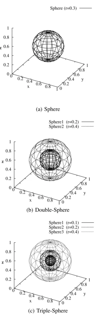
A. Two-category Classification Problems

First, we perform two-category classification problems as in Fig.2 to investigate the basic feature of the proposed method and to compare it with the SIRMs model. In the classification problems, points on [0,1]×[0,1]×[0,1] are classified into two classes: class 0 and class 1. The class boundaries are given as spheres centered at (0.5,0.5,0.5). For Sphere, the inside of sphere is associated with class 1 and the outside with class 0. For Double-Sphere, the area between Spheres 1 and 2 is associated with class 1 and the other area with class 0. For triple-Sphere, the inside of Sphere1 and the area between Sphere2 and Sphere3 is associated with class 1 and the other area with class 0. The desired outputyr

p is set as follows: ifxpbelongs to class 0, thenypr= 0.0. Otherwise

yr

(4)

0 0.2

0.4 0.6

0.8 1 0

0.2 0.4 0.6

0.8 1

0 0.2 0.4 0.6 0.8 1

z

Sphere (r=0.3)

x

y z

(a) Sphere

0 0.2

0.4 0.6

0.8 1 0

0.2 0.4

0.6 0.8

1

0 0.2 0.4 0.6 0.8 1

z

Sphere1 (r=0.2) Sphere2 (r=0.4)

x

y z

(b) Double-Sphere

0 0.2

0.4 0.6

0.8 1 0

0.2 0.4

0.6 0.8

1

0 0.2 0.4 0.6 0.8 1

z

Sphere1 (r=0.1) Sphere2 (r=0.2) Sphere3 (r=0.4)

x

y z

(c) Triple-Sphere

[image:4.595.85.252.86.638.2]

Fig. 2. Two-category Classification Problems

TABLE I

INITIAL CONDITION FOR SIMULATION.

A B (k= 1) B (k= 2) C

Tmax 10000 100 3000 3000

Kw 0.05 0.01 0.01 0.01

Kh - 0.05 0.05 0.05

Kc 0.00001 0.001 0.0001 0.0001

Kb 0.00001 0.001 0.0001 0.0001

TABLE II

SIMULATION RESULT FOR TWO-CATEGORY CLASSIFICATION PROBLEM.

Sphere Double-Sphere Triple-Sphere

A 1.699 1.562 2.753

(189) 2.210 4.320 5.412

B(k=1) 11.230 16.835 16.328

(30) 11.237 16.789 16.371

B(k=2) 1.484 2.128 3.476

(138) 2.179 5.095 6.307

C 1.660 4.550 5.019

(122) 3.317 8.582 8.789

TABLE III

INITIAL CONDITION FOR SIMULATION.

A B (k= 1) B (k= 2) C

Tmax 10000 100 1000 1000

Kw 0.01 0.01 0.01 0.01

Kh - 0.05 0.05 0.05

Kc 0.001 0.001 0.001 0.001

Kb 0.001 0.001 0.001 0.001

B. Obstacle avoidance

1) Obstacle avoidance: From (operation) data given by

an examinee to avoid obstacle, fuzzy inference rule for each model is constructed. As shown in Fig.3, the distance d and the angle θ between mobile object and obstacle are selected as 2 input variables. The mobile object moves with the vector A=(Ax, Ay) at each step, where the element

Ax of A is constant and the element Ay of A is only determined as an output from fuzzy inference. Learning data to avoid obstacle given by an examine are shown as 100 points in Fig.4. From the data, fuzzy inference rule to perform the trace of Fig.4 is constructed for each model, where the simulation condition is shown in Table III. The number of partitions for each model is 5. Fig.5 shows the results for the moves of mobile object from the starting places

at(0.1,0),(0.2,0),· · ·,(0.8,0),(0.9,0). In both SIRMs and

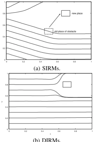
DIRMS models, obstacle avoidance is successful as shown in Fig.5. Further, test simulations with the place of obstacle different from the place in learning are performed with the same fuzzy inference rule for each model. As shown in Fig.6, the results are successful for both models.

2) Obstacle avoidance and arriving at the designated

place: As shown in Fig.7, the distanced1 and the angleθ1

y

0 x

d

vector A

obstacle

Ax Ay

[image:4.595.312.540.589.755.2]

mobile object

(5)

0 0.2 0.4 0.6 0.8 1

obatacle start place

[image:5.595.347.504.52.291.2]

learning data

Fig. 4. Learning data denoted by dots, to avoid obstacle.

0 0.2 0.4 0.6 0.8 1

(a) SIRMs.

0 0.2 0.4 0.6 0.8 1

y

x

[image:5.595.55.286.52.217.2]

(b) DIRMs.

Fig. 5. Simulation result for obstacle avoidance starting from various places learning

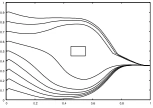
between mobile object and obstacle and the distanced2and the angleθ2between mobile object and the designated place are selected as input variables. The problem is to construct fuzzy inference rule that mobile object avoids obstacle and arrives at the designated place. From (operation) data, fuzzy inference rule for each model is constructed as shown as 200 points in Fig.8. The number of partitions for each model is 5. As the same method as the above, the mobile object moves with the vector A at each step. where Ay of A is output variable. The simulation condition is shown in Table III. The simulation results for SIRMs and DIRMs models are unsuccessful and successful, respectively, as shown in Fig.9. Fig.9 shows the results of moves of mobile object for starting places at (0.1,0),(0.2,0),· · · ,(0.8,0),(0.9,0) after learning. In Fig.9(a), mobile agent collides with ob-stacle in simulation of starting place at (0.4,0). Further, test simulations with the places, (1, 0.35), different from the designated place in learning are performed for DIRMs. The results are also successful in DIRMs model as shown in Fig.10. Lastly, we performed the same simulations for the

0 0.2 0.4 0.6 0.8 1

old place of obstacle new place

(a) SIRMs.

0 0.2 0.4 0.6 0.8 1

y

x

(b) DIRMs.

Fig. 6. Simulation for obstacle avoidance placed at different place after learning.

y

0 x

d

vector A

obstacle

Ax Ay

mobile object

goal

d2

[image:5.595.95.245.252.491.2]

2 1 1

Fig. 7. Simulation on obstacle avoidance and arriving at the goal.

constructive DIRMs model. As a result, all simulations are also successful in the constructive DIRMs. Therefore, the number 6 of modules for DIRMs model can be reduced to the model composed of 3 modules.

V. CONCLUSION

[image:5.595.311.536.336.508.2]

(6)

0 0.2 0.4 0.6 0.8 1

y

x

learning data

obstacle

[image:6.595.59.282.72.227.2]

The designated place

Fig. 8. Learning data to avoid obstacle and arrive at the designated place (1, 0.35).

0 0.2 0.4 0.6 0.8 1

(a) SIRMs.

0 0.2 0.4 0.6 0.8 1

[image:6.595.93.247.303.550.2]

(b) DIRMs.

Fig. 9. Simulation for obstacle avoidance and arriving at the different designated place after learning.

0 0.1 0.2 0.3 0.4 0.5 0.6 0.7 0.8 0.9 1

0 0.2 0.4 0.6 0.8 1

Fig. 10. Simulation for obstacle avoidance with the different designated place (1, 0.35) from learning.

two variables at a time as EX-OR problem. As a future work, we will consider theoretical characterization of SIRMs and DIRMs models.

REFERENCES

[1] H. Nomura, I. Hayashi and N. Wakami, A Self-Tuning Method of Fuzzy Reasoning by Delta Rule and Its Application to a Moving Obstacle Avoidance, Journal of Japan Society for Fuzzy Theory & Systems, vol.4, no.2, pp. 379–388, 1992 (in Japanese).

[2] C. Lin and C. Lee,Neural Fuzzy Systems, Prentice Hall, PTR, 1996. [3] S. Araki, H. Nomura, I. Hayashi and N. Wakami, A Fuzzy Modeling

with Iterative Generation Mechanism of Fuzzy Inference Rules,Journal of Japan Society for Fuzzy Theory & Systems, vol.4, no.4, pp.722–732, 1992.

[4] S. Fukumoto, H. Miyajima, K. Kishida and Y. Nagasawa, “A Destructive Learning Method of Fuzzy Inference Rules”,Proc. of IEEE on Fuzzy Systems, pp.687–694, 1995.

[5] H. Nomura, I. Hayashi and N. Wakami, A Learning Method of Simplified Fuzzy Reasoning by Genetic Algorithm,Proc. of the Int. Fuzzy Systems and Intelligent Control Conference, pp.236–245, 1992. [6] L.X. Wang and J.M. Mendel, Fuzzy Basis Functions, Universal

Approx-imation, and Orthogonal Least Square Learning,IEEE Trans. Neural Networks, vol.3, no.5, pp.807–814, 1992.

[7] S. Fukumoto and H. Miyajima, Learning Algorithms with Regular-ization Criteria for Fuzzy Reasoning Model, Journal of Innovative Computing, Information and Control, vol.1, no.1, pp.249–263, 2006. [8] J. Yi, N. Yubazaki and K. Hirota, A Proposal of SIRMs Dynamically

Connected Fuzzy Inference Model for Plural Input Fuzzy Control,Fuzzy Sets and Systems, 125, pp.79–92, 2002.

[9] N. Shigei, H. Miyajima and S. Nagamine, A Proposal of Fuzzy Inference Model Composed of Small-Number-of-Input Rule Modules,

Proc. of Int. Symp. on Neural Networks: Advances in Neural Networks - Part II, pp.118–126, 2009.

[image:6.595.94.247.627.735.2]