Fully Bayesian Source Separation of Astrophysical
Images Modelled by Mixture of Gaussians
Simon P. Wilson, Ercan E. Kuruo˘glu
, Senior Member, IEEE
, and Emanuele Salerno
Abstract—We address the problem of source separation in the presence of prior information. We develop a fully Bayesian source separation technique that assumes a very flexible model for the sources, namely the Gaussian mixture model with an unknown number of factors, and utilize Markov chain Monte Carlo tech-niques for model parameter estimation. The development of this methodology is motivated by the need to bring an efficient solu-tion to the separasolu-tion of components in the microwave radiasolu-tion maps to be obtained by the satellite mission Planck which has the objective of uncovering cosmic microwave background radiation. The proposed algorithm successfully incorporates a rich variety of prior information available to us in this problem in contrast to most of the previous work which assumes completely blind separation of the sources. We report results on realistic simulations of expected Planck maps and on WMAP 5th year results. The technique sug-gested is easily applicable to other source separation applications by modifying some of the priors.
Index Terms—Bayesian source separation, cosmic microwave background (CMB) radiation, Gibbs sampling, Markov chain Monte Carlo, Planck satellite mission.
I. INTRODUCTION
O
NE OF THE most important discoveries of the past century was undoubtedly the observation by Penzias and Wilson of the cosmic microwave background (CMB) radiation in 1964 [1]. It carries immensely important information about the universe and therefore it is of tremendous importance to make a full sky measurement of CMB. To date, two satel-lites—COBE [2] and WMAP [3]—have made measurements of extraterrestrial microwaves at several frequencies across the whole sky, with a third—Planck—to be launched in 2008 [3]. An important problem is that the signals measured by these satellites do not contain only CMB radiation but also contributions from a number of other sources.In this paper, a fully Bayesian source separation method is de-veloped to identify the CMB from observations of extraterres-trial microwaves made at several frequencies. This allows prior
Manuscript received January 31, 2008; revised August 08, 2008. Current ver-sion published December 10, 2008. This work was supported by the EU Net-work of Excellence MUSCLE, http://www.musclenoe.org, under FP6-507752, and in part by the Italian Space Agency, within the project “Studio di Cos-mologia e Fisica Fondamentale.” The associate editor coordinating the review of this manuscript and approving it for publication was Dr. Amir Leshem.
S. P. Wilson is with the Department of Statistics, Lloyd Institute, Trinity Col-lege Dublin, Dublin 2, Ireland (e-mail: [email protected]).
E. E. Kuruo˘glu and E. Salerno are with Istituto di Scienza e Tecnologie dell’Informazione, Consiglio Nazionale delle Ricerche, Pisa, Italy.
Color versions of one or more of the figures in this paper are available online at http://ieeexplore.ieee.org.
Digital Object Identifier 10.1109/JSTSP.2008.2005320
knowledge on these sources to be incorporated in the separa-tion process. A novel feature of our approach is the modeling of the sources by Gaussian mixture models (GMM) with an un-known number of factors, thus allowing for very rich prior mod-eling of sources. Prior distributions are specified for the GMM parameters. Other prior information that can be modelled is on the contribution of the different sources at different frequencies. Model assessment, by comparing observed data with a fitted model prediction, is also done. Our model also allows, by an easy extension, for the possibility of modelling dependencies between sources through generalizing the prior to multivariate Gaussian mixture models.
The posterior distribution is computed by Monte Carlo sam-pling. Another novel feature of this work is the use of the re-versible jump method of [4] to sample the GMM parameters. The separated sources are estimated as averages of the samples from the posterior distribution. Beyond this, further informa-tion can be extracted from the samples if desired, such as es-timates of uncertainty in the separation, like the standard devi-ation point-wise of the source samples, or functions of interest like the mean of the spectral density of the samples. The ability to do this is one of the principal benefits of the Bayesian ap-proach.
Various work over the last decade has addressed the CMB problem in a source separation framework. In particular, [5] modelled the problem as a noiseless linear mixture and solved this source separation problem using a gradient descent algo-rithm. Later, this work was extended to the full sky in [6] who used FastICA [7], a fast fixed point-algorithm. In [8] and [9], the emphasis is on separation in the frequency domain with the motivation of obtaining the angular spectrum of CMB directly. A spectral decomposition is computed for each source in the angular spectrum domain and then fitted to the observations using the expectation-maximization (EM) method. Later, [10] extended this work so that it could analyze data with missing patches through the use of wavelets.
A Bayesian approach to this problem was discussed in [11], where an entropic prior was proposed for the sources. Such a prior regularizes the separation such that the most plausible (highest entropy) sources are obtained from the data among all plausible ones. This work was generalized to the case of spa-tially varying noise and spectral properties of foreground com-ponents in [12]. However, the problem in this case was consid-ered as pure source reconstruction and not model learning, since the mixing matrix was assumed to be perfectly known. Refer-ence [13] proposed adopting a generic model, namely GMM for the sources and suggested independent factor analysis for the solution. This approach has assumed fixed but unknown model parameters which were learned using either EM algorithm or
simulated annealing (SA). This was extended in [14] to adopt prior distributions for model parameters hence moving to a fully Bayesian model. The resulting model was learned with Gibbs sampling. The work in this paper can thus be considered as an ideal logical continuation of [13], for the data model, and [14], for the sampling approach.
The estimation method proposed in [15] is at present the most similar to the one described in this paper, since it shares the data model and the sampling approach. Both data models, in par-ticular, assume a given parametric form for each source emis-sion spectrum. Note, however, that [15] assigns a uniform prior distribution to both the sources and the model parameters and bases the estimation strategy on an information criterion, as in [16]. Very recent unpublished work by the same authors has ex-tended the work to include nonuniform priors [17] where the power spectrum is estimated together with the spatial signal. In this work, the spatial signal is the focus and a faster convergence and a lower computational complexity is expected. We assume a Gaussian mixture prior for foreground signals while [17] sample jointly from a multivariate Gaussian prior.
In this work, we jointly estimate by sampling all unknowns in the model—sources, mixing matrix, and other parameters—and propose to use Gaussian mixtures with an unknown number of factors to model the sources. This prior distribution is a highly flexible prior model that can model any continuous probability distribution to arbitrary accuracy, thus, at least in principal al-lowing any information about the marginal distribution of the sources over the sky to be incorporated.
The rest of the paper is structured as follows. In Section II we give a brief description of the sources and the antenna noise. Based on this information, Section III gives the model for the mixing problem and describes the hierarchical Bayesian model that we use, including the priors we assume for the sources. Sec-tion IV describes the MCMC approach we use for the inference on the model we proposed. Section V provides simulation re-sults on both synthetic Planck images and real WMAP images. Finally, we provide a discussion of the results in Section VI.
II. SOURCES
The sources of radiation in the universe can be divided into three groups. The first is the CMB, which is observable in all di-rections from earth. The second are sources originating from in-side the galaxy and the third are extragalactic sources that orig-inate outside the galaxy.
A. CMB
The physics of CMB is very well studied and understood the-oretically [18], [19]. It is widely accepted that CMB is Gaussian, although recently there has been some debate on the deviation of CMB from Gaussianity. In this paper, we assume, as does most of the literature, that CMB is Gaussian. It is also widely expected to be stationary, as validated on WMAP data in [20], and that CMB anisotropies can be represented as the multipli-cation of a spatial template with a nonlinear function of the fre-quency.
For the recovery of certain cosmological parameters, it is con-venient to work in the angular spectrum domain and the CMB angular spectrum has a well known structure with a number of
peaks [19]. The CMB sources used in this work for the simu-lation example in Section V are generated synthetically using the HEALPIX software package, which assumes a spatially flat standard inflationary cold dark matter model with a Gaussian realization.
B. Galactic Components
a) Synchrotron:Synchrotron radiation is generated by elec-trons spiralling (hence accelerating) through magnetic fields. The synchrotron map that we use in the simulation example is a commonly used one in the literature, taken from the 408 MHz Haslam survey and extrapolated and scaled to Planck frequen-cies [21].
b) Galactic dust:Galactic dust is made up of small particles which range from the order of nanometers to micrometers. Their radiation is dominant especially in very high frequency chan-nels.
c) Free-free emission:Free-free or “Bremsstrahlung” emis-sion is caused by the colliemis-sion of free electrons with heavy ions in the ionized medium. Electrons lose energy in these collisions and emit photons.
C. Extragalactic Sources
d) Sunyaev–Zeldovich effect:The Sunyaev–Zeldovich (SZ) effect is generated by the inverse Compton scattering of photons from CMB on electrons.
e) Point sources:Point sources are caused by distant stars or galaxies which appear as localized, impulsive bursts of radia-tion. Unlike the sources discussed above, they are not diffuse and their impulsive behavior cannot be modelled with a GMM [22]. It is not possible to consider templates that scale in dif-ferent frequencies and each channel needs to be considered sep-arately. Due to these properties, the general approach in the lit-erature is to detect and remove them from radiation maps before starting the component separation task [23]. In this paper, we do not consider point sources and the Sunyaev-Zeldovich effect.
III. MODEL
The observation model consists of microwave amplitudes at frequencies over the sky at pixels. The data are denoted , . The source model consists of sources and is represented by the vectors , with each component representing the amplitude of a distinct phys-ical source of those microwaves. We assume that the follow a standard statistical independent components analysis model, so that they can be represented as a linear combination of the
(1)
where is an “mixing” matrix and is a vector of independent Gaussian error terms with precisions (inverse
vari-ances) . For convenience, define ,
to be the values of the th source over all pixels, and
(2) (3)
For the application to CMB separation, it is reasonable to pa-rameterize with a vector of considerably smaller dimension; see Section III-B. We write the mixing matrix as to em-phasize this point. We assume that each source is independent, defined by a prior distribution with parameters .
The goal is to estimate , the parameters
associated with the models for , and , given observation of . The noise variances are assumed known; for the Planck mis-sion, this is reasonable because of knowledge of the antenna. The independent components model between the and is also an example of a factor analysis model. In particular, we propose to use GMMs to represent the non-Gaussian sources, in which case it is an example of a model known as a mix-ture of factor analyzers [24]. In contrast to [24], in this work the mixtures are defined for the sources, rather than over both the mixing matrix and sources, since we do not necessarily want to place any physical interpretation on the different mixture fac-tors, for which different mixing matrix values might be reason-able. Rather, the purpose of the GMM is to provide flexible modelling of non-Gaussian sources. Like in [24], we adopt a Bayesian approach to data fitting but implemented by MCMC rather than the variational Bayes approach used there. We also assume that the number of factors in the GMM of each source is unknown.
Bayesian inference will be based on the posterior distribution, which following the above description can be factorized as
(4)
In the next few subsections, each element of this distribution is defined in turn [see (5), (10), (11) and (12)].
A. Noise Structure
The error primarily rises from detector noise and can be reasonably assumed to be independent and identically distributed Gaussian distributed with zero mean. The errors are mutually independent within and between pixels and frequency, and are assumed to be identically distributed at each frequency with precision . Most source separation studies, where noise is modeled, have assumed this.
A simple form of stochastic spatial dependence for the noise is assumed because the noise variance is dependent on the number of observations at each point in the sky [13]. This number may differ, according to the scanning schedule adopted by the detector. The number of measurements at pixel is assumed known to be where , is taken to be the mean of the measurements at each frequency and, since the mean of independent and identically distributed Gaussian random variables is also Gaussian with a precision that is times larger, this implies that the precisions of are . The term in (4) is therefore written as
(5)
where is the th row of . We do not explicitly define any spatial dependence between the directly, such as through a Markov random field model.
B. Mixing Matrix Structure for Astrophysical Microwave Sources
Each column of pertains to a source, and each row to a microwave frequency. Some restrictions are usually placed on in order to force a unique solution; factor analysis can only estimate and up to a permutation. Typically, in source separation studies for this application, this is achieved by setting one row of to be ones, e.g., [25]. There are no possible permutations that respect this restriction on and hence we have a unique solution. The first row is chosen arbitrarily to be ones.
There is a considerable amount of physical theory and obser-vation about the sources. This has led to models for how much each source contributes a different frequency that define a pa-rameterized relationship between the frequency and contribu-tion. It is the parameters of these models that make up . Each column of is the contribution to the observation of a source at different frequencies, and hence this is written as a function of the frequencies and . These parameterizations are approxima-tions that come from the current state of knowledge about how the microwaves for each source are generated. Here, we merely state the parameterization that we are going to use, and refer to [15], [26] and the many references therein for a more detailed exposition on the background to them.
It is assumed that the CMB is the first source and therefore, it corresponds to the first column of . It is modelled as a black body at a temperature (see [27]), and hence its contribution is a known constant at each frequency of the form
(6)
where
is the average CMB temperature, is the Planck constant and is Boltzmann’s constant. The ratio
is taken merely to ensure that , in line with our policy of constraining the first row of to be ones.
Next, we define for the synchrotron radiation column to be
(7)
where the spectral index, is typically in the range ( 2.3, 3.0) [28].
The column of that corresponds to galactic dust is of the following form [26]:
where and is the unknown spectral index for dust. We have assumed a range of (1,2) for .
The fourth column of , devoted to free-free emission is like that for synchrotron [26]
(9)
where is thought to lie in the range ( 2.3, 3.0).
C. Sources
The distribution of , source at pixel , is modeled as a GMM with an unknown number of factors . This provides a very flexible but tractable class of models for the sources.
De-fine , , and
to be the mixture factor means, precisions and weights for the th source. Hence, the parameters of the th
source are and
(10)
, where . Let
, , , and
denote the vectors of all mixture means, precisions, weights and number of factors for all the sources,
so that .
D. Priors
The remaining terms in (4) are and .
For , we use the conjugate prior dis-tributions [29, ch. 2] that facilitate the computation of the pos-terior and yet are flexible enough to incorporate good prior in-formation. The conjugate prior distributions mean that the dis-tributions that must be sampled from in the implementation by MCMC are of the same distribution type and so easy to generate from. Given , the prior distributions for the means
are assumed to be independent and identical Gaussian distributions with means and precisions , the prior distribution of the precisions are assumed to be independent and identical gamma distributions with shapes and scales and the prior distribution of the weights is assumed to be a Dirichlet distribution with equal parameters . The number of factors is assigned a geometric prior with mean , hence
(11)
Values must be specified for the prior distribution parameters: , , , , , and , for . They are assigned values to reflect what is known currently about the values of the sources. So if past studies for dust indicated a factor centred at 0.02 and another centred at 0.04 then we could assign
and . This prior specification follows [4], who discuss how to specify these values in more detail.
As mentioned in Section III-B, rough bounds on the values of the spectral indices are known. We use independent normal distributions for each
(12)
with mean and standard deviation so that 95% of the prior probability lies within the rough bounds. For example, the synchrotron spectral index is believed to lie in the range ( 2.3, 3.0), which leads to a normal prior with mean 2.65 and stan-dard deviation 0.175.
IV. IMPLEMENTING THESOURCESEPARATION
The source separation is implemented in two stages as fol-lows. The first stage is Monte Carlo sampling of the poste-rior distribution of (4), specifically by a Markov chain Monte Carlo method (MCMC) [30]. We do this rather than approxi-mate (4) by a variational approach, as in [24], because of con-cerns about the underestimation of posterior variance with vari-ational methods [31]; since one of the principal advantages of the Bayesian approach is the availability of estimates of uncer-tainty, we opted for the more computationally intensive MCMC. Once this is done, the second stage is to compute the average of the samples of the sources; this average is taken to be the esti-mated source.
An easy to implement MCMC scheme to sample from (4) is the Gibbs sampler, with some block updating e.g. we repeatedly sample from the full conditional distributions of blocks of the unknown variables. In many cases the full conditional distribu-tions are of known form, while in other cases they are sampled by a Metropolis step within the Gibbs sampler [32], [33]. The full conditional distributions that are sampled from in one iter-ation of the MCMC scheme are defined below.
f) Sampling : The full conditional distribution of each is [from (4)]
(13)
which after some manipulation is seen to be a GMM of
factors with precisions , means
and weights , for . The are conditionally independent over pixels for each source, so we sample each
separately, for and . It is easy to
simulate a value from this GMM by choosing a factor with the probabilities then sampling from the Gaussian distribution of the chosen factor.
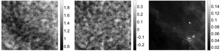
Fig. 1. Simulated example. Original CMB, synchrotron, and galactic dust patches all in milli Kelvins.
Fig. 2. Simulated example. Observations (in milli Kelvins) on the 3 of the 9 Planck channels: 30 Ghz (lowest frequency), 143 GHz (middle frequency), and 857 GHz (highest frequency).
full conditional distribution by a Metropolis step. Given the cur-rent value , is proposed from a Gaussian distribution with mean ; all other components of are kept constant. The new proposed mixing matrix is denoted to reflect the fact that only , and hence the th column of , is changed by the proposal. Then is sampled from the full conditional dis-tribution of (13) using . The set is jointly accepted or rejected. The accept probability is defined in (16) in the Appendix.
h) Sampling : To sample these
pa-rameters we follow the reversible jump MCMC method of [4]. Each source is updated separately. Associated with each source is a vector of mixture factor indices , , that assign each pixel to a partic-ular factor of the Gaussian mixture. The sampling is then
done on , which turns out to lead to
full conditional distributions of all the variables that are of a known type and easy to simulate. Briefly, the means are sampled from Gaussian distribution with means and precisions , where is the number of pixels assigned
to factor in e.g. . To avoid
the label-switching problem associated with fitting mix-ture models [34], the means are constrained to be ordered . The sample is regarded as a Metropolis proposal and is rejected if this ordering is not maintained. The precisions are sampled from gamma
distributions with scale and
shape . The weights are updated jointly from a Dirichlet distribution with parameters . The allocations are sampled from the discrete distribution
for . Finally, the number of factors can change by a Metropolis move that proposes to either split or merge a factor, then either create a new or delete an existing empty factor (one for which ). For these proposals, re-allocation of some existing pixels to new factors, and proposals for new
means, variances, and weights, must take place. We refer to [4] for the details of these, and the associated accept probabilities for the proposals.
V. EXAMPLES
A. Simulation Study
The first example is a 512 512 patch of realistic data that have been synthetically generated (CMB) or generated from previously reconstructed sources of synchrotron and dust, as discussed in Section II. These sources are shown in Fig. 1. Ob-servations were generated at 9 channels at the frequencies to be observed by Planck (30, 44, 70, 100, 143, 217, 353, 545, and 857 GHz), using the mixing matrix model of Section III-B with spectral indices and . The measurement error standard deviations used were 0.00126, 0.00120, 0.00113, 0.00028, 0.00018, 0.00018, 0.00018, 0.00018, and 0.00018 mK at each channel, respectively, which are those that are expected to be attained by the Planck detectors. Three of these maps are shown in Fig. 2.
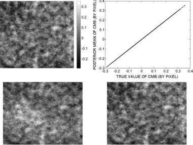
[image:5.594.113.478.181.268.2]Fig. 3. Simulated example. The posterior mean reconstruction of the CMB (in milli Kelvins) based on 5000 samples from the MCMC procedure (top left) with a scatter plot of true versus posterior mean (top right). On the bottom is the reconstruction of CMB by Fast ICA (left) and SMICA (right).
Fig. 4. Temperatures (in milli Kelvins) a 20 square patch of the sky from WMAP at 5 microwave frequencies.
Fig. 3 shows the average of the last 5000 samples of CMB, along with a scatter plot of these means against the true value, as shown in Fig. 1. We see from the scatter plot and from compar-ison with Fig. 1 that the CMB is very well reconstructed here. The same is true for the other two sources. Also in Fig. 3 is the reconstruction of CMB due to Fast ICA [7] and SMICA (spec-tral matching ICA) as in [35]. For Fast ICA, we used tanh as the approximation for non-Gaussianity and found that careful choice of a non-Gaussian model was necessary to get a good separation. SMICA requires a square mixing matrix, and the best result in terms of the lowest square error with the true CMB (from using the 30 GHz, 44 GHz, and 857 GHz channels) is shown. For SMICA, synchrotron is not separated at all,
prob-ably because we have used channels where only CMB and dust dominate. Although results for both Fast ICA and SMICA are not fully optimized with respect to all tuning parameters, the ap-proach of this paper is clearly producing a more accurate recon-struction over all sources. It is also noted that the reconstructed sources appear to show spatial correlation, even though this is not modelled. This is due to the spatial dependence pattern in the data.
B. Analysis of a WMAP Year 5 Patch
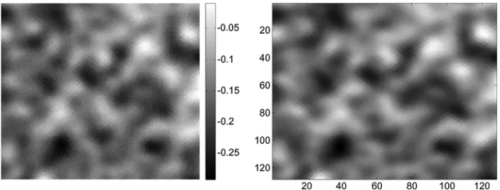
Fig. 5. Average of the last 10 000 samples of CMB (left) and a reconstruction from the WMAP team (right) in milli Kelvins.
Fig. 6. Posterior means of synchrotron, dust, and free-free emission in milli Kelvins.
some recently released five-year WMAP data at 20 north, 60 west, consisting of 128 128 pixels.
The algorithm of Section IV was implemented with four sources (CMB, synchrotron, dust and free-free emission). The noise precisions were assumed to be the published values for WMAP’s detectors. The spectral density for free-free emis-sion was fixed at 2.14 (following [15]). The priors for the synchrotron and dust spectral indices were the same as those for the simulated example, as were the priors for the number of factors in the GMM source models. Informative priors were placed on the GMM parameters, based on discussions on the expected marginal properties of the sources. For example, the prior distributions of the GMM parameters for CMB were
, , , and . This corresponds to a
Gaussian prior distribution for the CMB mean with mean 0 and variance 0.01, and a gamma prior distribution on the CMB precision with mean 0.05 and standard deviation 0.05.
The MCMC algorithm was run for 50 000 iterations. To check for adequate convergence and mixing, trace plots, auto-correla-tion funcauto-correla-tions and the Gelman-Rubin diagnostic [36] were com-puted over two runs of the MCMC from different starting values. Trace plots showed that the algorithm appeared to have con-verged in 20 000–30 000 iterations for the values of the sources, although the spectral indices were taking a longer time to con-verge. Autocorrelations were also low for the sampled values of the sources. The Gelman Rubin diagnostic was computed using the last 10 000 iterations of the two runs, and in general were between 1.2 and 1.6, but with the diagnostic for over 2, indicating some lack of convergence for the parameters of the mixing matrix. However, this does not seem to affect the sources; they appear to converge once the values of the spec-tral indices are close to convergence. Nevertheless, it is clear from these statistic values that getting better convergence of the MCMC is an important issue for future work.
Fig. 7. Posterior distribution of CMB intensity at pixel (20,20) in the patch.
[image:7.594.303.548.352.551.2]Fig. 8. Assessment of model fit. Scatter plots of the observed value ofd against the standardized residual over all pixels at the five frequencies.
had only one factor. This is probably due to the small size and homogeneous behavior of the data in the patch and is consistent with our prior belief that a small number of factors would be sufficient.
For model assessment, Fig. 8 is a scatter plot of the observed values against the standardized residuals
where
is the posterior expectation of under the model, obtained by taking the average of over the MCMC samples. A good model fit is indicated by a lack of trend in the plot, and values of the residual consistent with the standard normal distribution, e.g., rarely outside the interval ( 3,3). There is one figure for each frequency . These plots show a satisfactory fit of the data to the model; a separation consistent with the data has been produced, with no significantly large residuals or systematic unexplained trend in the residuals being displayed.
VI. DISCUSSION ANDFURTHERWORK
A fully Bayesian source separation algorithm for multi-channel image data has been presented, where sources are modelled as GMMs. The algorithm performs very well on sim-ulated Planck data and has been applied to data from WMAP.
Current work is on obtaining full sky maps for different sources using the WMAP 5th year data, so that angular spec-trum of CMB will be constructed as well. The results of this study will be presented in a follow up publication. For this reason, inference for the CMB power spectrum [38] is not
discussed. However, once such a map is sampled by MCMC then it is a straightforward matter to compute the posterior distribution of the power spectrum and summary statistics of it as follows. For each MCMC sample of the CMB, the power spectrum is computed. Then from this set of “samples” of power spectra, a pointwise sample mean can be taken as the best posterior estimate of the power spectrum. Uncertainty in the power spectrum can be quantified by computing, for example, the (2.5,97.5) sample percentiles pointwise.
see [39]. The cost of producing a map at ever-finer resolution is higher uncertainty in the reconstruction. This is because, for any observed resolution, subsampling at finer resolutions leads to samples with higher variance because there are more degrees of freedom under the constraints on their sum. We note that this idea of sub-sampling has been used with considerable success in many applications, including image data, e.g., [40].
Several generalizations are possible. An important model as-sumption, that is assumed in all model-based source separa-tion approaches to date, is thata priorisources are independent from each other. While our results show that such dependencies clearly exist in the posterior distribution, due to the stochastic linear constraint that , prior modelling of them should help to produce a more realistic separation. As we stated in the Introduction, this is a relatively straightforward extension of the model by allowing the source priors to be mixtures of multi-variate Gaussians; the posterior distribution of (4) remains the same except the term is now a mixture of multivariate Gaussian distributions for each pixel.
Another assumption is that a source is spatially uncorre-lated. Spatial dependence is most conveniently modelled by a Gaussian Markov random field and we have done some preliminary work on this idea [41]. Combining with cross source correlations, one might ultimately consider a mixture of multivariate Gaussian Markov random fields as a prior for the sources. Implementing the analysis with such a prior would be a significant challenge computationally; we hypothesize that it will be difficult to derive a well-behaved MCMC approach. Other functional approximations, such as that of [42], offer feasible alternative to computing the posterior distribution in this case.
Generalizing the relationship between sources and data to be nonlinear presents no difficulties either, at least in principle; it merely implies a replacement of the linear term in (5) with the desired nonlinear function . However, depending on the nature of the nonlinearity, satisfactory convergence and mixing of the MCMC for the parameters can become slow and difficult to confirm. Such a generalization would be useful in the galactic plane, where the relationship between sources and observation is not well understood but is certainly not linear be-cause of the interaction, such as absorption and re-emission, by the different causes of the galactic sources.
Finally, although the technique was developed for the astro-physical source separation problem in mind, it is general and is applicable to other source separation problems as well.
APPENDIX
In this Appendix, we derive the accept probability for the joint proposal of in the MCMC method described in Sec-tion IV.
The target distribution is the joint full conditional distribu-tion of and , which depends only on , (all the other sources except for ), and the normal mixture param-eters for . Given the current value , is proposed from a normal distribution with mean ; all other components of are kept constant. The new proposed mixing matrix is denoted
to reflect the fact that only , and hence the th column of , is changed by the proposal. Then is sampled from the full conditional distribution of (13) using . The accept probability for such a move is the usual target distri-bution ratio times proposal distridistri-bution ratio, that is to say the minimum of 1 and
The full conditional of is, from the relevant
ele-ments of (4), given by .
For the ratio of full conditionals of to , we must be careful since these are full conditionals that are conditional on different values of . Since
, so
Thus, the accept probability is the minimum of 1 and
(14)
where we have also substituted the uniform prior for . The integrand is the product of a Gaussian likelihood term (see (5)) and Gaussian mixture terms
[see (10)].
After rearranging the exponent term to isolate the , can be written
(15)
which, after expanding the exponent and completing the square, we can write as shown in the first equation at bottom of page next page, where the constants that we have ignored do not concern us as they do not depend on , and so will cancel out when we take the ratio in the accept probability.
equation at bottom of page. We now see that the integral is that of a Gaussian mixture over a Gaussian mean (treating as the “mean”); standard results show this to be another Gaussian with variance as the sum of the two Gaussians in the integral (e.g. the
sum and and mean as the mean of
the mixing Gaussian (e.g. in this case, will be replaced by ). Thus we have (16), shown at the bottom of the page. Sub-stituting (16) into (14) gives the required accept probability.
REFERENCES
[1] A. Penzias and R. Wilson, “A measurement of the flux density of Cas A at 4080 mc/s,”Astrophy. J. Lett., pp. 1149–1154, 1965.
[2] NASA, Cobe homepage [Online]. Available: http://lambda.gsfc.nasa. gov/product/cobe/
[3] NASA, Planck Surveyor homepage [Online]. Available: http://map. gsfc.nasa.gov/
[4] S. Richardson and P. Green, “On Bayesian analysis of mixtures with an unknown number of components (with discussion),”J. R. Statist. Soc. B, vol. 59, pp. 731–792, 1997.
[5] C. Baccigalupi, L. Bedini, C. Burigana, G. D. Zotti, A. Farusi, D. Maino, M. Maris, F. Perotta, E. Salerno, L. Toffolatti, and A. Tonazzini, “Neural networks and the separation of cosmic microwave background and astrophysical signals in sky maps,”Monthly Notices R. Astron. Soc., vol. 318, pp. 769–780, 2000.
[6] D. Maino, A. Farusi, C. Baccigalupi, F. Perotta, A. J. Banday, L. Be-dini, C. Burigana, G. D. Zotti, K. M. Gorski, and E. Salerno, “All-sky astrophysical component separation with fast independent component analysis,”Mon. Not. R. Astron. Soc., vol. 334, no. 1, pp. 53–68, 2002.
[7] A. Hyvarinen, “Fast and robust fixed-point algorithms for indepen-dent component analysis,”IEEE Trans. Neural Networks, vol. 10, pp. 636–634, May 1999.
[8] H. Snoussi, G. Patanchon, J. Macias-Peres, A. Mohammad-Djafari, and J. Delabrouille, “Bayesian blind component separation for cosmic mi-crowave background observations,” inAIP Proc. Maximum Entropy and Bayesian Inference Conf., 2001, pp. 125–140.
[9] J. Delabrouille, J.-F. Cardoso, and G. Patanchon, “Multidetector mul-ticomponent spectral matching and applications for cosmic microwave background data analysis,”Mon. Not. R. Astron. Soc., vol. 300, pp. 1–29, 2003.
[10] Y. Moudden, J. F. Cardoso, J. L. Starck, and J. Delabrouille, “Blind component separation in wavelet space: Application to cmb analysis,”
EURASIP J. Appl. Signal Process., vol. 2005, no. 15, pp. 2437–2454, 2005.
[11] M. P. Hobson, A. W. Jones, A. N. Lasenby, and F. R. Bouchet, “Fore-ground separation methods for satellite observations of the cosmic mi-crowave background,”Mon. Not. R. Astron. Soc., vol. 300, pp. 1–29, 1998.
[12] V. Stolyarov, M. P. Hobson, A. N. Lasenby, and R. B. Barreiro, “All-sky component separation in the presence of anisotropic noise and dust temperatute variations,”Mon. Not. R. Astron. Soc., vol. 357, pp. 145–155, 2005.
[13] E. E. Kuruo˘glu, L. Bedini, M. T. Paratore, E. Salerno, and A. Tonozzini, “Source separation in astrophysical maps using indepen-dent factor analysis,”Neural Networks, vol. 16, pp. 479–491, 2003. [14] E. E. Kuruo˘glu and P. Milani Comparetti, “Bayesian separation of
inde-pendent sources in astrophysical radiation maps using mcmc,” inProc. Statistical Problems in Particle Physics, Astrophysics and Cosmology, L. Lyons, Ed., 2003, pp. 321–323.
[15] H. K. Eriksen, C. Dickinson, C. R. Lawrence, C. Baccigalupi, A. J. Banday, K. M. Górski, F. K. Hansen, P. B. Lilje, E. Pierpaoli, K. M. Smith, and K. Vanderlinde, “CMB component separation by parameter estimation,”Astrophys. J., vol. 641, pp. 665–682, 2006.
[16] A. R. Liddle, “How many cosmological parameters?,”Mon. Not. R. Astron. Soc., vol. 351, pp. L49–L53, 2004.
[17] H. K. Eriksen, J. B. Jewell, C. Dickinson, A. J. Banday, K. M. Górski, and C. R. Lawrence, Joint Bayesian Component Separation and CMB Power Spectrum Estimation arXiv, Tech. Rep. astro-ph/0709.1058v2, 2008.
[18] M. White and J. D. Cohn, “The theory of anisotropies in the cosmic microwave background,”Amer. J. Phys., vol. 70, no. 2, pp. 106–118, 2002.
[19] W. Hu and S. Dodelson, “Cosmic microwave background anisotropies,” Annu. Rev. Astron. Astrophys., vol. 70, no. 2, pp. 106–118, 2002.
[20] E. Komatsuet al., “First year Wilkinson microwave anisotropy probe (wmap) observations: Tests of Gaussianity,”Astrophys. J. Suppl. Se-ries, vol. 148, pp. 119–134, 2003.
[21] C. G. T. Haslam, C. J. Salter, H. Stoffel, and W. E. Wilson, Astrophys. J. Suppl. Series, vol. 47, pp. 1–143, 2006.
[22] D. Herranz, E. E. Kuruo˘glu, and L. Toffolatti, “An alpha-stable ap-proach to the study of the p(d) distribution of unresolved point sources in cmb sky maps,”Astron. Astrophys., vol. 424, pp. 1081–1096, 2004. [23] M. Tegmark, D. J. Eisenstein, W. Hu, and A. de Oliveira-Costa, “Ac-curate removing point sources from cosmic microwave background maps,”Astrophys. J., 1998.
[24] Z. Ghahramani and M. Beal, “Variational inference for Bayesian mixtures of factor analysers,” in Advances in Neural Informa-tion Processing Systems, T. K. L. S. A. Solla and K.-R. Müller, Eds. Cambridge, MA: MIT Press, 2000, vol. 12, pp. 449–455. [25] L. Bedini, D. Herranz, E. Salerno, C. Baccigalupi, E. E. Kuruo˘glu, and
A. Tonazzini, “Separation of correlated astrophysical sources using multiple-lag data covariance matrices,” EURASIP J. Appl. Signal Process., vol. 15, pp. 2400–2412, 2005.
[26] M. Tegmark, D. J. Eisenstein, W. Hu, and A. de Oliveira-Costa, “Fore-grounds and forecasts for the cosmic microwave background,” Astro-phys. J., 2000.
[27] J. C. Mather, D. J. Fixsen, R. A. Shafer, C. Mosier, and D. T. Wilkinson, “Calibrator design for the cobe far infrared absolute spectrophotometer (FIRAS),”Astrophys. J., vol. 512, pp. 511–520, 1999.
[28] P. Reich, W. Reich, and J. C. Testori, “Spectral index variations of galactic emission,” The Magnetised Interstellar Medium B. Uyaniker, W. Reich, and R. Wielebinski, Eds., 2003, pp. 63–70.
[29] P. M. Lee, Bayesian Statistics: An Introduction, 3rd ed. London, U.K.: Hodder Arnold H&S, 2004.
[30] A. E. Gelfand and A. F. M. Smith, “Sampling based approaches to calculating marginal densities,”J. Am. Statist. Assoc., vol. 85, pp. 398–409, 1990.
[31] B. Wang and D. M. Titterington, “Variational Bayes estimation of mixing coefficients,” in Deterministic and Statistical Methods in Machine Learning, Lecture Notes in Artificial Intelligence. New York: Springer-Verlag, 2005, vol. 3635, pp. 281–295.
[32] A. Gelman, J. B. Carlin, H. S. Stern, and D. B. Rubin, Bayesian Data Analysis, 2nd ed. London, U.K.: Chapman & Hall, 2003.
[33] W. Hastings, “Monte Carlo sampling methods using Markov chains and their applications,”Biometrika, vol. 57, pp. 97–109, 1970. [34] G. Celeux, “Bayesian inference for mixtures: The label-switching
problem,” inProc. COMPSTAT, R. Payne and P. Green, Eds., 1998, pp. 227–232.
[35] J.-F. Cardoso, H. Snoussi, J. Delabrouille, and G. Patanchon, “Blind separation of noisy Gaussian stationary sources. Application to cosmic microwave background imaging,” in Proc. EUSIPCO, 2002, pp. 561–564.
[36] A. Gelman and D. B. Rubin, “Inference from iterative simulation using multiple sequences,”Statist. Sci., vol. 7, pp. 457–472, 1992. [37] G. Hinshaw, J. L. Weiland, R. S. Hill, N. Odegard, D. Larson, C.
L. Bennett, J. Dunkley, B. Gold, M. R. Greason, N. Jarosik, E. Komatsu, M. R. Nolta, L. Page, D. N. Spergel, E. Wollack, M. Halpern, A. Kogut, M. Limon, S. S. Meyer, G. S. Tucker, and E. L. Wright, Five-year Wilkinson Microwave Anisotropy Probe (WMAP) Observations: Data Processing, Sky Maps & Basic Results NASA, Goddard Space Flight Center Tech. Rep., 2008 [Online]. Available: http://lambda.gsfc.nasa.gov/product/map/dr3/pub/_pa-pers/fiveyear/basic_results/wmap5basic.pdf.
[38] P. F. Scott, P. Carreira, K. Cleary, R. D. Davies, R. J. Davis, C. Dick-inson, K. Grange, C. M. Gutiérrez, M. P. Hobson, M. E. Jones, R. Kneissl, A. Lasenby, K. Maisinger, G. G. Pooley, R. Rebolo, J. A. R. no Martin, P. J. S. Molina, B. Rusholme, R. D. E. Saunders, R. Savage, A. Slosar, A. C. Taylor, D. Titterington, E. Waldram, R. A. Watson, and A. Wilkinson, “First results from the very small array—III. The cosmic microwave background power spectrum,”Mon. Not. R. Astron. Soc., vol. 341, pp. 1076–1083, 2003.
[39] A. E. Gelfand, A. Mugglin, and B. P. Carlin, “Fully model based ap-proaches for misaligned spatial data,”J. Amer. Statist. Assoc., vol. 95, pp. 877–887, 2000.
[40] D. Higdon, H. Lee, and Z. X. Bi, “A Bayesian approach to character-izing uncertainty in inverse problems using coarse and fine-scale in-formation,”IEEE Trans. Signal Processing, vol. 50, pp. 389–399, Feb. 2002.
[41] K. Kayabol, E. E. Kuruo˘glu, and B. Sankur, Bayesian Separation of Images Modelled With Markov Random Fields Using MCMC ISTI, Consiglio Nazionale delle Ricerche Tech. Rep., 2008.
[42] H. Rue, S. Martino, and N. Chopin, “Approximate Bayesian inference for latent Gaussian models using integrated nested Laplace approxima-tions,”J. R. Statist. Soc. B, 2008.
Simon P. Wilsonwas born in Newcastle upon Tyne, U.K., in 1968. He received the Ph.D. degree from George Washington University, Washington, DC, in 1994.
He is currently an Associate Professor with the School of Computer Science and Statistics, Trinity College Dublin, Ireland. He has been a Postdoctoral Researcher with the National Institute of Standards and Technology (NIST), Gaithersburg, MD, a Vis-iting Researcher with the École Polytechnique, Paris, France, and INRIA-Sophia Antipolis, and a Visiting Professor with the Universidad Carlos III, Madrid, Spain. His research interests are in application of Bayesian statistical methods to data analysis problems in science and engineering, particularly in image processing, reliability and telecommunications.
Ercan E. Kuruo˘glu(S’89–M’98–SM’06) was born in Ankara, Turkey, in 1969. He received the B.Sc. and M.Sc. degrees in electrical and electronics en-gineering from Bilkent University, Turkey, in 1991 and 1993, and the M.Phil. and Ph.D. degrees in infor-mation engineering from the Signal Processing Lab-oratory, Cambridge University, Cambridge, U.K., in 1995 and 1998, respectively.
Upon graduation from Cambridge, he joined the Collaborative Multimedia Systems Group, Xerox Re-search Center, Cambridge. In 2000, he was in INRIA-Sophia Antipolis, with the Ariana Project as an ERCIM Fellow. In 2002, he joined ISTI-CNR, Pisa, Italy, as a Permanent Member. Since 2006, he has been an Associate Professor and Senior Researcher. He was a Visiting Professor with the Georgia Institute of Technology graduate program, Shanghai, China, in Autumn 2007. He was a Visiting Researcher/Lecturer for extended periods in Bogazici University, Izmir Institute of Technology, Turkey, University of Cantabria, Spain, Xidian University and Shanghai Jiao Tong University, China. He is the author of more than 60 peer reviewed publications and holds four U.S. and European patents. His research interests are in statistical signal processing and information and coding theory with applications in image processing, as-tronomy, telecommunications, intelligent user interfaces and bioinformatics.
Dr. Kuruo˘glu was an Associate Editor for the IEEE TRANSACTIONS ON
SIGNAL PROCESSING from 2002 to 2006. He is currently on the editorial board of Digital Signal Processing and is an Associate Editor for IEEE TRANSACTIONS ON IMAGE PROCESSING. He guest-edited special issues in various journals on heavy tailed processes, cosmology applications of signal
processing, and Bayesian source separation. He was the Special Sessions Chair for EURASIP European Signal Processing Conference, EUSIPCO 2005, and was the Technical co-Chair for EUSIPCO 2006. He is also an elected member of the IEEE Technical Committee on Signal Processing Theory and Methods.
Emanuele Salerno graduated in electronic engi-neering from the University of Pisa, Italy, in 1985.
In 1987, he joined the Italian National Research Council as a full-time Researcher. At present, he is a Senior Researcher with the Signals and Im-ages Laboratory, Institute of Information Science and Technologies, Pisa. He has been working in applied inverse problems, image reconstruction and restoration, microwave nondestructive evaluation, and blind signal separation, and held various re-sponsibilities in research programs in nondestructive testing, robotics, numerical models for image reconstruction and computer vision, and neural network techniques in astrophysical imagery. He has been supervising various theses in computer science, electronic and communications engineering, and physics, and, since 1996, has been teaching courses at the University of Pisa.