Fast Approximate Inverse
Bayesian Inference in
non-parametric Multivariate
Regression
with application to palaeoclimate reconstruction
A thesis submitted to the University of Dublin, Trinity College
in partial fulfillment of the requirements for the degree of
Doctor of Philosophy
Department of Statistics, School of Computer Science and Statistics
University of Dublin, Trinity College
April 2009
Declaration
This thesis has not been submitted as an exercise for a degree at any other
Univer-sity. Except where otherwise stated, the work described herein has been carried out
by the author alone. This thesis may be borrowed or copied upon request with the
permission of the Librarian, University of Dublin, Trinity College. The copyright
belongs jointly to the University of Dublin and Michael Salter-Townshend.
Michael Salter-Townshend
Abstract
Bayesian statistical methods often involve computationally intensive inference pro-cedures. Sampling algorithms represent the current standard for fitting and test-ing models. Such methods, while flexible, are computationally intensive and suffer from long run times and high potential sampling error. New methods for fitting non-parametric approximations offer a fast and accurate alternative. Essentially, a multivariate Gaussian distribution is used to approximate the posterior of the model parameters.
Cross-validation is a useful tool in model validation which is an important as-pect of statistical inference. Sampling based methods require many re-runs and are impractical for this task. A new method is developed in this thesis that performs fast cross-validation using the Gaussian approximations.
Study of the palaeoclimate provides insight into long-term climate variability. This represents the motivating problem for the work in this thesis. A probabilistic forward model for vegetation given climate is fitted to modern training data using Bayesian methods. The model is then inverted and inference on climate given fossil pollen counts may be performed; this is referred to as the inverse model and cross-validation is preferred in this context.
Highly multivariate models may sometimes be broken down into a sequence of independent smaller problems, which may then be dealt with more easily in parallel. Procedures for assessing the performance of this approach are developed for the inverse problem via fast cross-validation.
Acknowledgements
My first acknowledgement is to my supervisor, Professor John Haslett. Although this is no surprise (I have yet to see an acknowledgements section for a thesis that did not start with a supervisor) I must emphasize that John has done a good deal more for me than most supervisors would and a great more than his job description would suggest.
John is a functioning collection of seemingly contradictory things; he is both enthusiastic and patient, wise and humble, serious and fun. He has begun to teach me that it is possible to appreciate the big picture and the minute details of a complex problem at the same time. Without this unique set of attributes I have no doubt that I would not have lasted long in statistical research.
John has guided me through a crisis of confidence when I felt that I had nothing to contribute. He has been both friend and mentor. However, it is in the day-to-day supervisory capacity that he has excelled most. When I look back at the range of errors and shortcuts I have attempted to get past him it is bewildering how he has managed to supervise me with a smile and to gently guide me back towards the correct path.
Secondly, I thank Professor H˚avard Rue, of NTNU in Trondheim, Norway. I visited H˚avard in Norway twice in 2007 for a total of three productive months and was made to feel welcome. H˚avard’s knowledge of statistics seems almost limitless and the rapidity with which he has always replied to inquiries is astounding. His new methods and approximations are central to this thesis and will no doubt become used in a wide variety of statistical problem. H˚avard contributed much discussion in the formulation of the zero-inflated model presented in the thesis.
not only accepted my self afflicted impoverishment but has fed and clothed me on occasion. Most importantly, I have never had difficulty in leaving work in the lab as coming home to Emma is coming home to the most beautiful girl in the world, which tends to re-focus my attention...
I thank my family, in particular my parents, who have part financed my PhD time and are always proud and encouraging. I have always been assured that there is no problem on which I cannot seek their help and advice.
I acknowledge Science Foundation Ireland and Enterprise Ireland for the funding that paid for my time with John. The Norwegian Government Scholarship pool paid for one of the visits to Trondheim.
Michael Salter-Townshend
University of Dublin, Trinity College
Contents
Abstract iii
Acknowledgements iv
List of Tables xi
List of Figures xii
Publications xiv
Chapter 1 Introduction 1
1.1 Palaeoclimate Reconstruction Project . . . 2
1.1.1 The RS10 Pollen Dataset . . . 2
1.1.2 Response Surfaces . . . 2
1.1.3 The Classical Approach . . . 3
1.1.4 The Bayesian Approach . . . 4
1.2 Computational Challenges . . . 7
1.3 Overview of Chapters . . . 7
1.4 Research Contributions . . . 11
Chapter 2 Literature Review and Statistical Methodology 12 2.1 Palaeoclimate Reconstruction Literature Review . . . 12
2.1.1 Classical Approach . . . 14
2.1.2 Bayesian Approach . . . 15
2.2 Relevant Bayesian Methods . . . 18
2.2.1 Bayesian Hierarchical Model . . . 19
2.2.3 Directed Acyclic Graphs . . . 21
2.2.4 Gaussian Markov Random Fields . . . 21
2.3 Integrated Nested Laplace Approximations . . . 25
2.4 Spatial Zero-Inflated Models . . . 27
2.4.1 Single Process Model for Zero-Inflation . . . 29
2.5 Inverse Regression . . . 31
2.5.1 Non-parametric Response Surfaces . . . 31
2.5.2 Toy Problem Example . . . 32
2.6 Model Validation . . . 38
2.6.1 Inverse Predictive Power . . . 38
2.6.2 Cross-Validation . . . 39
2.7 Conclusions . . . 41
2.7.1 Advances in this Thesis . . . 42
Chapter 3 Models with Known Parameters 43 3.1 The Univariate Problem . . . 44
3.1.1 Given New Counts Data . . . 46
3.1.2 Given Training Data Only . . . 46
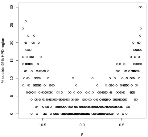
3.1.3 Percentage Outside Highest Predictive Distribution Region . . 46
3.2 Disjoint-Decomposable Models . . . 49
3.2.1 The Marginals Model . . . 51
3.2.2 Non-Disjoint-Decomposable Models . . . 52
3.2.3 Sources of Interaction . . . 54
3.3 Multivariate Normal Model . . . 56
3.3.1 General Case Normal Models . . . 56
3.3.2 Sensitivity to Dependence . . . 60
3.4 Counts Data . . . 62
3.4.1 Poisson Model . . . 62
3.4.2 Scaled Poisson . . . 62
3.4.3 Overdispersion . . . 64
3.4.4 Sensitivity to Zero-Inflated Likelihood . . . 65
3.5 Compositional Data . . . 66
3.5.2 Dirichlet Distribution . . . 69
3.5.3 Generalized Dirichlet Distribution . . . 70
3.5.4 Logistic-Normal Class of Distributions . . . 70
3.5.5 Multivariate, Constrained Likelihood Functions . . . 72
3.5.6 Nested Compositional Models . . . 74
3.5.7 Disjoint-Decomposing Compositional Models . . . 84
3.6 Conclusions . . . 85
3.6.1 Disjoint-Decomposition of Models . . . 86
3.6.2 Zero-Inflated Models . . . 86
3.6.3 Nested Constrained Models . . . 87
Chapter 4 INLA Inference and Cross-Validation 88 4.1 The Integrated Nested Laplace Approximation . . . 89
4.1.1 The Gaussian Markov Random Field Approximation . . . 90
4.1.2 Spatial Zero-Inflated Counts Data . . . 98
4.1.3 Posterior for the Hyperparameters . . . 101
4.1.4 Laplace Approximation for Parameters . . . 103
4.1.5 Approximation for Parameters: Inverse Problem . . . 104
4.2 Cross Validation . . . 105
4.2.1 Importance Resampling . . . 107
4.2.2 Cross-Validation in Inverse Problems . . . 108
4.2.3 Fast Augmentation of the Multivariate Normal Moments . . . 109
4.2.4 More Computational Savings . . . 115
4.2.5 Summary Statistics of Model Fit . . . 116
4.2.6 Toy Problem Example . . . 116
4.3 Conclusions . . . 117
Chapter 5 Inference Methodology 121 5.1 Reasons for Disjoint-Decomposition . . . 122
5.1.1 Parallelisation . . . 122
5.1.2 Memory Usage . . . 122
5.1.3 Inverse Problem . . . 123
5.2 Multivariate Normal Model . . . 124
5.2.1 Conditions for Perfect Disjoint-Decomposition . . . 125
5.2.2 Compositional Independence . . . 127
5.3 Sensitivity to Inference via Marginals . . . 128
5.3.1 Discrete HPD Regions . . . 132
5.3.2 Nested Constrained Models . . . 132
5.4 Conclusions . . . 135
Chapter 6 Application: the Palaeoclimate Reconstruction Project 137 6.1 Bayesian Palaeoclimate Reconstruction Project . . . 137
6.1.1 The RS10 Dataset . . . 138
6.1.2 Software and Hardware . . . 140
6.2 Model Description . . . 141
6.2.1 Cross-Validation . . . 144
6.2.2 Fast Inversion of the Forward Model . . . 145
6.2.3 Buffer Zone for Inverse Problem . . . 145
6.3 Zero-Inflation . . . 145
6.4 Results . . . 149
6.4.1 Treatment of Hyperparameters . . . 149
6.4.2 Marginals Model . . . 152
6.4.3 Uncertainty in Climate Measurements . . . 157
6.4.4 Zero-Inflated Model . . . 157
6.4.5 Nested Compositional Model . . . 159
6.4.6 Outliers . . . 163
6.5 Conclusions . . . 170
6.5.1 Advances . . . 170
6.5.2 Shortcomings . . . 171
Chapter 7 Conclusions and Further Work 173 7.1 Conclusions . . . 173
7.2 Further Work . . . 175
7.2.1 3 Dimensional Climate Space . . . 175
List of Tables
2.1 Numerical calculation of inverse stage . . . 35
5.1 Joint Precision matrix. . . 126
List of Figures
2.1 Directed Acyclic Graph . . . 22
2.2 Univariate response: forward and inverse . . . 33
2.3 Results for various model parameters . . . 37
3.1 Examples of easy, medium and hard for given new data . . . 47
3.2 Examples of easy, medium and hard; general new data . . . 48
3.3 Disjoint-Decomposable Model . . . 52
3.4 % outside 95% HPD region against number of surfaces modelled . . . 53
3.5 Non-Disjoint-Decomposable Models . . . 54
3.6 Error as a Function of Interaction . . . 63
3.7 Inverse Predictive Distributions: Zero-Inflated Counts . . . 67
3.8 The Simplex Space . . . 68
3.9 Nested Compositions: Example . . . 75
3.10 Nested Compositions: Example . . . 76
3.11 Nested Compositions: Simplest Case . . . 77
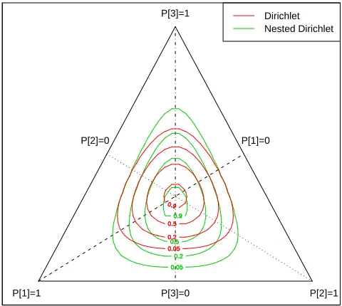
3.12 Prior Nested Dirichlets . . . 79
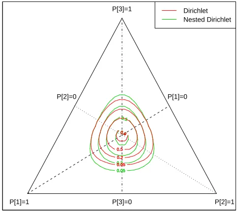
3.13 Posterior Nested Dirichlets . . . 80
3.14 % outside 95% HPD region; repititions and density, high overdispersion 82 3.15 % outside 95% HPD region; repititions and density, low overdispersion 83 4.1 Quadratic Approximation to Poisson . . . 92
4.2 Gaussian Univariate Approximation . . . 95
4.3 Quadratic Approximation to Zero-Inflated Poisson . . . 96
4.4 MCMC and GMRF Approximations: Zero-Inflated Poisson Likelihood 97 4.5 MCMC Chain Trace Plot: Log-rate . . . 98
4.7 Percentage of Points Outside 95% HPD: Zero-Inflation . . . 118
5.1 % outside 95% HPD region versus replications . . . 131
5.2 % outside 95% HPD region versus independent surfaces . . . 133
5.3 Convergence of inverse predictive distribution . . . 134
5.4 % outside 95% HPD region; repititions and density . . . 135
6.1 Modern climates; buffer zone . . . 146
6.2 Localised Histograms of Proportions Data . . . 150
6.3 Positive Abundances versus Probability of Presence . . . 151
6.4 Effect of using the modal hyperparameters . . . 153
6.5 Distribution of the ∆ statistic across taxa; Pollen dataset . . . 154
6.6 Plot of the ∆ statistic against number of taxaT . . . 155
6.7 Plot of the Dstatistic against number of taxa T . . . 156
6.8 Distribution of the Dstatistic; with and without Gaussian Blurring . 158 6.9 Structure of the Nesting of pollen dataset . . . 162
6.10 Distribution ofDlj, the expected squared distances to observations 164 6.11 Plot of the ∆ statistic against number of taxaT; within nest . . . 165
6.12 Example inverse cross-validation predictive distributions . . . 166
6.13 Inverse Predictive Densities: Extreme Outlier . . . 167
6.14 Outliers and altitudes; sample densities . . . 168
Publications
Some of the work presented in this thesis has been taken from the author’s following publications, which are co-authored as stated
Haslett J., Bhattacharya S., Whiley M., Salter-Townshend M., Wilson S., Allen J.R.M., Huntley B., and Mitchell F. (2006). Bayesian Palaeoclimate Reconstruction J. R. Statist. Soc. A. , 169, Part 3, 1–36.
Salter-Townshend M., and Haslett J. (2006) Zero-Inflation of Compositional Data, Proceedings of the 21st International Workshop on Statistical
Chapter 1
Introduction
Highly multivariate statistical problems may lead to slow inference procedures. One example of such a problem involves palaeoclimate reconstruction from fossil pollen data, which is an example of an inverse problem. Existing explorations of this chal-lenging area of study often involve a trade off between model complexity and speed of inference. Fast approximate Bayesian inference methods offer a solution. In addi-tion, an extension of the methodology allows for model validation to be performed quickly for the inverse problem. Conversely, the large scale of the palaeoclimate project offers a real challenge to the emerging approximate inference engine.
The Royal Statistical Society read paper “Bayesian Palaeoclimate Reconstruc-tion”, Haslett et al. (2006) presented work on high resolution pollen based recon-struction of the palaeoclimate at a single location since the last ice-age. This paper outlined the basic concepts involved in performing fully Bayesian inference on un-known climates given modern and fossil pollen data and modern climatic data. The work was a detailed “proof of concept”; extensions and improvements to the statis-tical methodology were considered, both in the paper and in the subsequent printed discussion.
1.1
Palaeoclimate Reconstruction Project
The Bayesian palaeoclimate reconstruction project is an ongoing initiative to build upon existing classical approaches to the reconstruction of prehistoric climates, using fossil pollen data. Specifically, the project seeks to handle all uncertainties quantita-tively and coherently in a fully Bayesian framework and to combine different types of information to reduce these uncertainties.
1.1.1
The RS10 Pollen Dataset
The primary dataset for the palaeoclimatology reconstruction project is the RS10 dataset of Allen et al. (2000). A collection of modern pollen surface sample counts
Ym
y
m
1 , . . . , yMm;M 7742 are taken from the uppermost 5 to 10mmof lake bed
sediment at numerous locations in the northern hemisphere. Along with covariates in the form of local contemporary climate measurements Lm, they comprise the
modern dataset. This is also referred to as the training data. Sample fossil pollen counts Yf are extracted from cores taken from lake or mire sediment. Measures of
the prehistoric climate variables Lf at the time of deposition of these fossil pollen
spores are unknown; the central premise of palynological palaeoclimate reconstruc-tion is that these climates may be inferred from the pollen data, albeit with some uncertainty. Both the modern and fossil pollen data comprise counts of numerous plant types (taxa; see below). There is therefore a vector of counts reported at each sampling location. The length of this vector is equal to the number of distinguishable pollen spore types.
1.1.2
Response Surfaces
Reconstruction of past climates involves using a multivariate regression type model in which the proportion of the ith species in the training pollen data set ym
i is an
indirect observation of a latent “response” to the corresponding modern climate variables Lm. This response is defined as the propensity to contribute pollen to the
second stage, the regression is “inverted” and applied to assemblages of fossil data, which yields a quantitative reconstruction of climate. The two stages are referred to as the forward and the inverse parts of the model respectively. This is known as
the response surface method.
Huntley (1993) argues that at least some species may have multiple optima and hence the response function may be multimodal. Non-parametric modelling of the response function is therefore advocated. This is due at least in part to the fact that the pollen data is in fact sorted into plant “taxa” rather than individual species. Each taxon consists of one or more species; sometimes an entire genus or even an entire family comprising several plant species are categorized simply as a single taxon. A given taxon may then contain multiple species that thrive and fail at dissimilar climates. This is because the pollen data are categorized visually and multiple related species frequently produce pollen spores that are indistinguishable to the eye.
1.1.3
The Classical Approach
There is a considerable literature on palaeoclimate reconstruction from such paly-nological data using the response surface methodology in the botany community (see for example Bartlein et al. (1986), Huntley (1993) and Allen et al. (2000)). These reconstructions use various estimation methods, essentially attributing to a fossil pollen assemblage the modern climate that has the “closest” matching pollen assemblage.
under very different climatic regimes. For a given fossil pollen assemblage, some of the 10 closest modern day responses may be steppe and some tundra; the averaged corresponding climates will lie in between in the climate space. This reconstructed climate may be in a region of climate that does not produce pollen assemblages anything like the fossil assemblage; it may even correspond to a climate that simply does not occur.
1.1.4
The Bayesian Approach
Unlike the classical approach, the Bayesian paradigm deals with all sources of un-certainty in a coherent manner. The unknown statistical parameters X are treated as random variables and a likelihood functionπYSXis used to express the relative
probabilities of obtaining different values of this parameter when a particular dataset
Y has been observed. Prior probability densities πX are placed on the unknown
parameters to reflect any subjective beliefs held before observation of data. The posterior density πXSYis delivered via Bayes theorem; it is a normalised product
of the prior and likelihood densities and reflects the updated beliefs in light of the data.
πXSY
πXπYSX
πY
πXπYSX
prior likelihood (1.1)
Bayes theorem constructs the posterior density πXSY which is a summary of
all knowledge about the parameter X subsequent to observing Y. The posterior distribution is a comprehensive inference statement about the model variables X. Any summary of the posterior distribution is useful e.g. moments, quantiles, highest posterior regions and credible intervals.
Forward Problem
In this stage of the inference, the modern training data of pollen counts and associ-ated climatic data are used to inform probabilistic statements on the unobservable response of vegetation to climate. The vectors of pollen counts at each location are modelled as indirect observations of the unknown responses 1 to the climate at that location. Building upon the notation already used in this section, the responses are labeled X There is a vector ofX responses at each point in the climate space, one for each taxon. Each individual taxon then has a set of responses across the climate space referred to as the taxon response surface; jointly over all taxa these are denoted by X.
Bayes theorem is used as above to construct the posterior for the response sur-faces given the modern data, Y
m, Lm
.
πXSY
m, Lm
πXπY
m
SL
m, X
πY
m
πXπY
m
SL
m, X
RXπ Y
m
SL
m, X
πXdX
(1.2)
The integral in the denominator is typically not tractable analytically. In Haslett et al. (2006) numerical integration was performed approximately using a Metropolis-Hastings Markov Chain Monte Carlo algorithm.
Inverse Problem
The second stage of the Bayesian inference procedure is the calculation of posterior probability distributions on the unknown palaeoclimates Lf, given the posterior for
the latent surfaces πXSY
m, Lm
(derived in the first stage of the model) and the
fossil pollen counts Yf. This is the inverse problem (also known as multivariate
non-linear calibration; ter Braak discussion of Haslett et al. (2006)).
Sampled responses X are passed to an MCMC algorithm for sampling from the posterior for palaeoclimate Lf given fossil pollen Yf and the surfaces X.
1Response here refers to the unobservable response of vegetation to climate only; it is the
πL
f
Sdata πL
f
SY
m, Yf, Lm
S π L
f, X
SY
m, Yf, Lm
dX
S π L
f
SX, Y
m, Yf, Lm
πXSY
m, Yf, Lm
dX
S π L
f
SX, Y
f
πXSY
m, Yf, Lm
dX (1.3)
As the fossil pollen counts alone (without knowledge of the climate at which they occurred) contribute little, or even no, information to the posterior for response surfaces given data, πXSY
m, Lm, Lf
is approximately equal to πXSY
m, Lm
:
S π
L
f
SX, Y
f
πXSY
m, Yf, Lm
dX S π
L
f
SX, Y
f
πXSY
m, Lm
dX (1.4)
The fully Bayesian approach is to solve the left-hand side of Equation (1.4); the right-hand side is an approximation that is common to most inverse problems.
In fact, a positive feedback mechanism may occur if the fossil counts are left in Equation (1.4); removing them may in fact lead to a more accurate fit. This is referred to as “cutting feedback”; Rougier (2008) states that cutting feedback, although technically a violation of coherence, may be presented in terms of best-input. The model is trained using only the data about which the analyst is confident. Essentially, fitting the responses using the modern training data, for which counts and climates are available, and the fossil data, for which counts only are available, may lead to unwanted positive feedback due to the fossil counts. The model training will begin by placing fossil counts in a region of climate space; given this selected region, the response surface appears to fit well. But the response surface was built using those counts in that region. The initial choice has been strengthened, despite the fact that is was an arbitrary choice. Training the model only on the modern data, for which climate is known, is preferred for this reason.
Integration over the latent surfaces was via Monte Carlo integration in Haslett et al. (2006): samples Xi, . . . , Xn are drawn from the posterior using the first stage
(forward problem) and passed to the second stage (inverse problem):
S π L
f
SX, Y
f
πXSY
m, Lm
dX
n
Qπ L
f
SXi, Y
f
An alternative to MCMC for this task is proposed in this thesis. Namely, the suite of approximation techniques referred to as INLA are applied and expanded for this purpose. The implications of imposing any new modelling procedures and algorithms on the forward stage are considered primarily in terms of the impact on the inverse stage.
1.2
Computational Challenges
The most pressing challenges encountered in the Bayesian palaeoclimate project to date involve the intensive computations necessary to carry out inference on the parameters of interest. This is due mainly to an over-reliance on the computationally intensive Markov Chain Monte Carlo algorithm. The large number of parameters required in the complex modelling leads to serious concerns about the mixing the algorithm achieves in the unknown parameter space. Linked to this is the problem that convergence is far from assured, even after runs of the order of weeks (see Haslett et al. (2006)). Additional detail in the model is prohibited due to memory and computation concerns.
As discussed briefly in Section 1.1.1, the unobservable response surfaces must be modelled non-parametrically. One way to achieve this is by discretising climate space on a regular grid and modelling the response as a random variable at each node. High resolution is desirable, requiring the use of a very fine discrete grid on the climate variable space. This results in a very large number of latent variables. The paper Haslett et al. (2006) dealt with a model including the order of 104 unknowns; and this is for a inference performed on a greatly reduced dataset using a simplified model.
1.3
Overview of Chapters
Chapter 2: Literature Review and Statistical Methodology
A brief review of the literature on palaeoclimate reconstruction is presented. Progress towards the standard set by Haslett et al. (2006) is charted and Bayesian statistical methods for inverse inference are summarised. The remaining weaknesses in the current methodology are outlined and the techniques used to overcome these in this thesis are introduced.
Chapter 3: Models with Known Parameters
In order to separate modelling issues from issues of inference in the forward problem, this chapter focusses on models with known parameters. Various model choices and the implications of these choices are presented. Some new statistical models are detailed. The novel contributions of this chapter are the methods for determining the decomposability of large, multivariate models into separate, independent modules and the nested compositional model. Issues related to the decomposition of models are introduced and discussed.
Chapter 4: INLA Inference and Cross-Validation
reconstruc-tion project, this may become computareconstruc-tionally overwhelming and is therefore not considered. Approximation methods are once again discussed in this context along with further application to the pollen / climate dataset.
Chapter 5: Inference Methodology
An investigation is carried out into the implications of decomposing the counts data vectors and carrying out marginal inferences on each component of the vector se-quentially. This is at best identical to a joint inference on all components at once and at worst an approximation to it. The accuracy of the approximation is expressed as a function of several impacting factors and the conditions for exact reproduc-tion of the joint posterior from the marginal posteriors (perfect decomposireproduc-tion) are described.
Details related to performing inference using the techniques already developed in previous chapters are presented. This chapter serves as a platform towards the application to real data in Chapter 6.
Chapter 6: Application: the Palaeoclimate Reconstruction Project
The motivating problem for the research conducted in this thesis is to improve and advance the palaeoclimate reconstruction project. Therefore, a chapter is devoted to applying the work developed in previous chapters to the RS10 pollen and climate dataset. The various approximation algorithms allow for a richer modelling of the forward problem (the response of vegetation to climate) than was previously possi-ble. The modelling of zero-inflation represents a fundamental change in the model. Practical issues regarding the application of the new model and use of the approxi-mations are identified and discussed. Results are presented and compared with the results derived from previous approaches. A fast cross-validation methodology for the inverse problem is central to this chapter.
Chapter 7: Conclusions and Further Work
1.4
Research Contributions
The following is a statement of the main contributions to the palaeoclimate recon-struction project by the author as presented in this thesis:
1. Investigation is conducted into the accuracy lost in sequential modelling of individual plant taxa responses to climate.
2. Nested compositional counts models for the palaeoclimate dataset are intro-duced. It is demonstrated that knowledge of the nesting structure is crucial to performing accurate inferences.
3. A fast Bayesian inference procedure on the forward stage of the palaeoclimate reconstruction model is demonstrated. This allows for far richer models to be developed and, more importantly, validated.
4. A model for parsimonious modelling of zero-inflation of the counts data that is compatible with the INLA methodology is presented.
Chapter 2
Literature Review and Statistical
Methodology
In order to set the context of the work in this thesis, a brief palaeoclimate reconstruc-tion literature review is conducted in Secreconstruc-tion 2.1. Gaps in the existing methodology are identified and solutions developed in this thesis are introduced.
The contributions are relevant to a wider statistical methodology beyond palaeo-climate reconstruction; Section 2.2 discusses Bayesian methods that are relevant to the methodology developed in this thesis. Section 2.4 introduces explicit modelling of zero-inflated counts data. Section 2.5 defines inverse regression and demonstrates the generic challenge of such problems with a simple example. Section 2.6 begins the discussion of how models of this type are evaluated and compared, focusing on inverse problems.
2.1
Palaeoclimate Reconstruction Literature
Re-view
Although the contributions made in this thesis to both statistical modelling and inference are applicable to a variety of problems, it is most natural to set them in the context of the motivating problem of statistical palaeoclimate reconstruction using pollen data.
con-ducted here in order to motivate and frame the work in this thesis.
Detailed reviews are already available; see ter Braak (1995) for a review of non-Bayesian palaeoecology, Haslett et al. (2006) for a review of Bayesian and non-Bayesian palaeoclimate reconstruction and Bhattacharya (2004) for details on Bayesian inference in inverse problems with a focus on palaeoclimate reconstruc-tion. It is not a worthwhile exercise to reproduce these in detail here; an overview, drawing directly from these and other sources is sufficient. Details may be found in the references.
The outline for the literature review is as follows:
Section 2.1.1 provides a brief review of non-Bayesian estimation methods in
the palaeoclimate literature. As per Haslett et al. (2006), these are referred to as “classical”. This section is relies on reference to the existing reviews in ter Braak (1995), Haslett et al. (2006), Bhattacharya (2004).
Section 2.1.2 deals mainly with the methodology of Haslett et al. (2006).
Re-lated Bayesian approaches are also discussed. Challenges and shortcomings in these techniques are identified.
Unfortunately, the terminology used in palaeoclimate statistics has become some-what confused. ter Braak (1995) categorises non-Bayesian approaches into two dis-tinct paradigms, which he terms “classical” and “inverse”. The former refers to regression of ecological data on climate. The latter is vice-versa; hence the label inverse as cause and effect have been inverted. “Classical” reconstruction may be thought of as building a forward (cause implies effect) model and subsequently in-verting the model to find cause given effect. This use of “inverse” reconstruction involves the simpler task of regression of cause (climate) on effect (ecology).
Haslett et al. (2006) and Bhattacharya (2004) do not consider the ter Braak (1995) definition of “inverse” modelling and use the term “classical” to refer to all non-Bayesian approaches. “Inverse” modelling in these works refers to the inversion of a forward model, Bayesian or otherwise. “Forward” models are equivalent to the models calibrated on the modern data in the “classical” approach of ter Braak (1995).
of “forward”, “inverse” and “classical” will be dropped from here on; the ter Braak (1995) definition of “inverse” will be referred to as classical inverse.
2.1.1
Classical Approach
ter Braak (1995) notes that palaeoclimate reconstruction is a highly non-linear mul-tivariate calibration problem. Although climate reconstruction from modern and fossil pollen is taken as the only worked example, the author notes that the tech-niques carry over immediately to calibration in other areas of palaeoecology.
He uses the interesting phrase
“the present day calibration is used to infer the past climate”
to broadly describe the way that all statistical climate reconstruction techniques work. The contribution of this thesis mainly lies in the calibration of such data (spatial, compositional, zero-inflated counts). The focus is in building and assessing the models.
It is worth noting that although Krutchkoff (1967) claims the superiority of this definition of the classical inverse method in predictive power, ter Braak (1995) shows that this approach is only slightly better when samples are from a large central part of the distribution of the training set. The inversion of the forward model is considerably better at the extremes. The classical inverse method also treats each climate variable separately and independently; a surprising and illogical model. In the Bayesian context, it is more natural to build forward (cause implies effect) models and invert using Bayes rule.
The classical palaeoclimate modelling approach may be split into three ap-proaches:
1. Response surfaces; polynomials and non-parametric
2. Analogue method;k nearest neighbours
3. Least squares type methods in classical inverse sense
Haslett et al. (2006) and developed here. Response surface methods typically use least squares based methods to regress pollen on climate; this relationship is then inverted to produce inference on fossil climate given pollen. Bartlein et al. (1986) used cubic polynomials in two climate dimensions fitted to observed percentages of eight pollen types. The authors encountered two difficulties with their approach:
1. some pollen type exhibited multimodal responses
2. the polynomials lacked flexibility and behaved strangely at the edge of the sample climate space.
Both of these problems were addressed through switching from fitting cubic polynomial response functions to non-parametric responses. Prentice et al. (1991) used local weighted averaging to fit smooth non-parametric surfaces to the data. This technique has since been followed by Huntley (1993) and others and is the closest non-Bayesian equivalent to the model of Haslett et al. (2006).
This method posed the question of what to do with the problem of multiple modern analogues. In fact, this problem is common for inverse problems (see Sec-tion 2.5.1). In the method of Allen et al. (2000), the locaSec-tions in climate space of the ten “nearest” response surface to the compositional fossil vector were averaged. This was an attempt to provide a single location as the most likely reconstructed climate. However, it can be a mostunsatisfactory approach; in the simplest example, a plant type that is abundant in the centre of climate space will send the signal “not close to centre” when the fossil record has low pollen counts of this type. The ten nearest response surface values will come from the edges of climate space. Averaging these ten locations in climate space will then reconstruct the centre; i.e. the very place that the signal most strongly rejects!
2.1.2
Bayesian Approach
which the pollen type is scarce; an honest assessment of belief in light of the low signal.
The Bayesian paradigm (Section 2.2) has been applied to palaeoclimate re-construction; however, the literature is “very small and scattered” (Haslett et al. (2006)). The first detailed Bayesian methodology comes from a series of papers by a group in the University of Helsinki (Vasko et al. (2000), Toivonen et al. (2001) and Korhola et al. (2002)). However, they work with a single climate variable and use a unimodal response with a functional form, invoking Shelford’s law of tolerance, which states that a species thrives best at a particular value of an environmental variable (optimum) and cannot survive if this variable is too high or too low.
Such a response model is inappropriate for many applications of ecology model. For example, Huntley (1993) shows that, for pollen data, multimodal responses in several climate dimensions are common. This is a result of species indistinguishably; most pollen spore types represent several species or even an entire genus.
More recent Bayesian work by Holden et al. (2008) also invoke Shelford’s law. This allows them to avoid MCMC based inference. In that paper, zero-inflation of the data is explicitly modelled; presence and abundance when presence are modelled as functions of a single underlying spatial process. This model is related to the model of Salter-Townshend and Haslett (2006).
Haslett et al. (2006)
Recognizing the issue with multimodal responses, Haslett et al. (2006) applied the non-parametric response surfaces approach of Huntley (1993) in a Bayesian context. A 5050 regular grid was employed across a two dimensional climate space on which
statistics were then used in lieu of theoretical ones.
Computation was found to be the main challenge of the methodology; this in turn led to restrictions on both the complexity of the model and, more importantly, in the validation procedures used to test and compare models. Due to these short-comings, the paper was presented as a “rather detailed proof of concept” Haslett et al. (2006). A section on issues deferred details some of the shortcomings and the printed discussion with the paper addresses several others.
The work contained in this thesis seeks to address some of these difficulties. Alternative inference techniques are employed, novel to the problem of palaeoclimate reconstruction, in place of the computationally overwhelming sampling algorithms used in Haslett et al. (2006). These techniques yield a normalised posterior on all parameters in closed form; see Section 2.3 for an introduction and Section 4.1 for full details. Assumptions made necessary by computational concerns may be relaxed, leading to a richer model posterior and the availability of more rigorous testing.
The final paragraph of the rejoinder from the authors of Haslett et al. (2006) to the contributed written discussion of the paper ended as follows:
“Zero inflation is a particular challenge . . . There may well be sampling procedures for the [parameters] that are more efficient than simple ran-dom sampling. In short, there remain many methodological challenges.”
In fact, while the authors acknowledge the need to treat the zero counts specially, the model they employ is one for overdispersion only, once again sacrificing model sophistication to computational efficiency.
The avoidance of intensive sampling algorithms allows for more sophisticated models to be developed. In particular, this thesis presents a new model for spatial zero-inflated counts data. The new model is flexible, yet simple. It offers a far more satisfactory account for the extra zeros in the data, yet remains parsimonious.
“predict” the data give a measure of model fit.
However, this would require fitting the model several thousand times. With running times of several weeks, after which the authors concede that “convergence to the correct posterior is far from assured”, repeating the procedure even a dozen times is undesirable to say the least. Therefore, the authors use an approximate cross-validation shortcut; the model, as fit to the entire dataset is used as an ap-proximation to the fit for each left-out point.
In contrast to this, constructing closed form posteriors, using new closed form techniques requires only a few minutes of run time. The development of these techniques is not a contribution in this thesis although application to the area of palaeoclimate reconstruction is novel. Re-fitting the model for each left-out point is now a realistic exercise. Another contribution in this thesis is to quickly correct the entire fitted model to account for leaving out a datapoint, rather than re-fit the model, thus achieving a fast inverse cross-validation.
2.2
Relevant Bayesian Methods
The Bayesian analyst is concerned with learning from a dataset about some unknown parameters. In the Bayesian framework, these parameters are treated as random variables and prior probability distributions are placed on these parameters. These reflect the analyst’s beliefs before seeing the data; they can be subjective and in-formed by personal and / or expert opinion, inin-formed by previous analysis of other datasets or totally uninformative, reflecting a complete ignorance or lack of belief.
The data are modelled using a likelihood function. This is a probability distribu-tion for the data, given the parameters. Using Bayes rule (given in Equadistribu-tion (1.1)), the prior and likelihood are multiplied to give an un-normalised posterior. This posterior, once normalised, gives a probabilistic distribution on the updated beliefs in light of the data. All useful summaries of knowledge subsequent to observation of the data may be calculated directly from the posterior distribution.
carried in the data but, for example, expert opinions too.
2.2.1
Bayesian Hierarchical Model
The general type of model considered in this thesis is a Bayesian hierarchical model (see Bernardo and Smith (1994) chapter 4). Hierarchical models have two or more levels of dependency. The hyperparameters θ specify the distribution of the latent parameters X which in turn specify the parameters of the likelihood functions for the dataY (this notation will remain consistent throughout). The hyperparameters themselves may in turn be modelled as random variables with a hyperprior.
Y πYSX
X πXSθ
θ πθ (2.1)
The level of data is called the first level, the parameters of the likelihood are level two and so forth.
2.2.2
Markov Chain Monte Carlo
Normalisation of the posterior is one of the primary challenges to implementation of the Bayesian method. In recent years, the use of Markov Chain Monte Carlo (MCMC) methods has become almost ubiquitous in Bayesian statistical inference, due largely to the availability of cheap and powerful computing resources (Gelfand and Smith (1990)). One common algorithm for performing MCMC based inference is the Metropolis-Hastings rejection sampling algorithm.
Iterative Metropolis-Hastings algorithms (introduced in Metropolis et al. (1953) and generalised in Hastings (1970)) generate a Markov chain of samples from any target probability distribution (such as the posterior in Equation (2.4)). The samples of the Markov chain can then be used to form any desired summary of the target distribution. The desired distribution only needs to be known up to a proportionality constant and therefore the denominator in Equation (2.4) is not required.
distribu-tion has density fX. Then, given a sample value of Xt, a proposed value X
is generated from a pre-specified proposal density qX
SXt and then accepted with
probability αXt, X
, given by
αXt, X
min1,
fX
qXtSX
fXt qX
SXt
¡ (2.2)
If the proposed value is accepted, the next sampled valueXt1 is set toX
. Oth-erwise, Xt1 is set to Xt. If a symmetric proposal distribution is used (for example
a random walk or an independence sampler), then the q terms in Equation (2.2) cancel. Looping over this procedure n times produces a Markov chain of samples
X1, . . . Xn fromfX, after convergence.
Constructing the algorithm is usually not difficult. Challenges are encountered when attempting to construct an algorithm that will return enough independent samples from the posterior to facilitate accurate inferences. MCMC methodology is plagued by the following issues.
1. Mixing: Due to the frequently high dimensionality of the space of parameters of interest a large number of independent samples is required to adequately describe the posterior distribution. The variables are often strongly depen-dent on each other and therefore sequential samples from the Markov chain are highly correlated. One-at-a-time updates suffer from poor mixing due to these correlations, unless an efficient multivariate proposal distribution can be constructed to perform joint updates. Mixing refers to the ability of the algorithm to explore the full support of the target distribution. Independence samplers for high dimensional spaces will lead to high rejection rates in the Metropolis-Hastings algorithm, greatly reducing the number of effective sam-ples.
In most practical problems a mixture of intuition, experience andad hocmethods are used to determine the length of an MCMC run required to generate a sufficient sample from the posterior. This is particularly challenging for the forward stage of the palaeoclimate reconstruction project due to the non-parametric modelling approach which necessitates a very large number of highly correlated variables.
2.2.3
Directed Acyclic Graphs
A directed acyclic graph, or DAG, is a powerful graphical tool for model building and illustration. A graph with directed arcs and no directed cycles is used to represent the model. The direction of the arcs gives the conditional dependencies.
Hierarchical models are most easily expressed using a DAG, where arrows be-tween each variable denote dependence. If, for example, a variable a depends on another variable b in a statistical model, then the DAG for this is simply a b.
Throughout this thesis, the structure of all models considered have an overall DAG corresponding to
θ X Y (2.3)
Each of the three levels may consist of multiple variables with extra dependency structure, suppressed in this simplified graph.
Bayesian inference procedures, such as those listed below, allow for inference on the distribution of the parameters given the data via Bayes rule:
πX, θSY
πYSX, θπX, θ
RX,θπ
YSX, θπX, θdX, θ
(2.4)
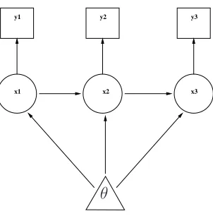
Bayesian Networks are probabilistic DAGs whose nodes represent random vari-ables. The directed arcs of the DAG denote the conditional dependencies of the model represented. For example, Figure 2.1 shows a DAG for a hierarchical model;
2.2.4
Gaussian Markov Random Fields
y1 y2 y3
x1 x2 x3
[image:36.612.224.375.17.170.2]θ
Fig. 2.1: An example directed acyclic graph, or DAG. The entire hierar-chical model is specified graphically; trivariate X depends on θ and each element is linked with the one to the right so that the model of X is, e.g. auto-regressive of order one, given θ. Data Y are observational modes that depend exclusively on the latent parameters X.
X to be incorporated into the model. One or more of the set of hyperparameters may be used to model the degree of covariance between these latent variables.
For a vector X defined in a discrete location space, a labeled graph G V, ω
defines the Markov structure ofX. V 1, . . . , nindexes the locations and ω is the
set of edges (dependency connections from one node to another) for each node of the graph. There is no edge between nodes i and j iff xiÙxjSx
i,j.
Definition 1 x x1, . . . , xn
T is a GMRF w.r.t. a labeled graph
G V, ω with
mean µ and precision matrix Q iff its density has the form
πx 2π
n
2
SQS
1
2exp
1
2xµ
TQ
xµ (2.5)
and
Qij x0i, j>ωfor all ixj (2.6)
Assigning a Markov structure to the latent field renders both the prior and posterior for the latent parameters to be a Gaussian Markov Random Field (GMRF) w.r.t. a graph G. The reason for using a Markov structure, as opposed to defining
If the precision (inverse covariance) matrix for the latent field is sparse, then fast numerical algorithms may be employed; details of this are described in Section 4.1. These Gaussian Markov random fields model the response surfaces of previous sec-tions as stochastically smooth across the location space.
If each node of the graph has an edge to all other nodes then the graph is said to
be fully connected. Assigning a regular Markov structure to the graph breaks many
of the edges resulting in a sparse precision matrix.
Discrete and Finite Space
The use of Markov random fields requires the location space to be defined on a discrete grid. Use of a fine grid blurs the distinction between discrete and continuous space. The data for locations may then be shifted to the nearest gridpoint or left as continuous and calculations at these locations may be evaluated cheaply as weighted averages of the values at the surrounding gridpoint values.
Intrinsic GMRFs
Intrinsic GMRFs are defined by an improper log-density. No mean is specified and the the precision matrix cannot therefore be inverted to give the covariance matrix. Intrinsic GMRF priors are often used for the parameters describing the latent surfaces. This allows for the specification of prior beliefs on the smoothness of the surfaces without specifying a prior mean.
Following Rue and Held (2005):
Definition 2 Let Q be a symmetric, positive semi-definite matrix with rank nkA
0, where k A 0 is the dimension of the null space of Q. x x1, . . . , xn
T is an
improper GMRF of rank nkA0 with parameters µ, Q if its improper density
is
πx 2π
nk
2
SQS
1
2exp
1 2x
TQx
(2.7)
whereSQS
is the generalized determinant ofQ(the product of the non-zero
eigen-values).
Chapter 3). In fact, the precision matrix for an intrinsic GMRF does not formally exist, however following Rue and Held (2005) the nn matrix Q with rank nk
(and kA0) is referred to as the precision matrix of the intrinsic GMRF.
An intrinsic GMRF of kth order is an improper GMRF of rank n
k, where PjQij 0 for all i. Hence, the conditional mean of xi is the weighted mean of its
neighbours, but has no specified overall level.
Random Walk
A convenient prior on a vector X whose indices are one dimensional may be derived from the random walk. For example, the first order random walk in one dimension is constructed from independent increments of X, defined on n discrete points (nodes on the graph G).
xixi 1
iid
N0, κ 1
(2.8)
which implies that
xjxi N0,jiκ 1
(2.9)
for i j. The full, joint density for X is then derived from its n1 increments
(πx1Sx0, . . . πxnSxn 1
where πxiSxi 1
Nxi 1, κ
1
) given by Equation (2.8) as (again, following Rue and Held (2005))
πXSκ κ n1~2
exp
κ
2
n1 Q
i 1
Dxi
2
κn1~2
exp
κ
2
n1 Q
i 1
xi 1
xi
2
κn1~2
exp
1 2X
TQX
(2.10)
S
1 1
1 2 1
1 2 1
1 2 1
1 2 1
1 1 (2.11)
Similar structure matrices may be constructed based on higher order random walks in any dimension of space, subject to edge effects. The imposition of a spatial structure models the latent surfaces as stochastically smooth using just a single hyperparameter κ. This hyperparameter controls the degree of spatial smoothing.
Link Functions
The parameters of many likelihood functions, particularly for counts data, require non-negative parameters. Link functions are therefore used to transform the unre-stricted latent field variables into positive numbers.
For example, if the data are modelled as Poisson, then the rates (positive) may be modelled as the exponents of multivariate Gaussian distributed random variables.
yi P oissonyi;λi
λi expxi
X GM RFX;µX, QX (2.12)
In this example the hyperparametersθare comprised of the means and precisions of the latent field, µX and QX.
2.3
Integrated Nested Laplace Approximations
πX, θSY
πYSX, θπX, θ
RX,θπ
YSX, θπX, θdX, θ
(2.13)
which is more conveniently expressed as
πXSθ, YπθSY
πYSX, θπXSθπθ
Rθ
RXπ
YSX, θπXSθdXdθ
(2.14)
The most common approach is to use MCMC to sample from the posterior for X and θ. This approach, while hugely popular, is not without its drawbacks (Sections 2.1.2 and 2.2.2). New techniques introduced in Rue and Held (2005) and developed further in Rue et al. (2008) offer a fast approximation called Integrated Nested Laplace Approximations (INLA).
Starting with the identity
πθSY
πX, θSY
πXSθ, Y
(2.15)
Replacing the denominator with a normalised Gaussian approximation evaluated at the mode (X
θ) yields
πθSY
πX, θSY
˜
πGXSθ, Y R R R R R R R R R R RX X
θ
(2.16)
This is known as the Laplace approximation for the hyperparameters. The Gaus-sian approximation for the latent field posterior, ˜πGXSθ, Y, is demonstrated in
detail in Section 4.1.
The basic procedure for INLA type inference on Bayesian hierarchical models is as follows:
The posterior for the hyperparameters is approximated using the Laplace
ap-proximate in Equation (2.16).
The posterior for the smooth latent field, given the data and hyperparameters,
is approximated by a GMRF at gridded / discrete values of the hyperparam-eters.
The approximate marginal posterior for the latent field, given the data only is
If the marginal value for a particular latent parameter (location in the field)
is required to a greater degree of accuracy, a Laplace approximation is built using a similar procedure to Equation (2.16).
Full details of how this is achieved and the relative strengths and weaknesses of the method are examined in Section 4.1. It is sufficient here to note that implemen-tation of these new methods is novel in the context of palaeoclimate research. They allow for increased sophistication in the forward model and more rigorous sensitivity analysis and model validation.
Contributions to the actual INLA methodology in this thesis consist of a method for performing fast updates to the entire posterior to correct for leaving out data; this has an immediate application in cross-validation in the inverse sense (see Sec-tion 2.6.2). Local correcSec-tions are sufficient for cross-validaSec-tion in the forward sense as the location is known in this case.
2.4
Spatial Zero-Inflated Models
Many counts datasets include zero-inflation; there are an excessive number of zero counts. Of particular interest is spatial data that exhibit such an overabundance of zeros. If these zero counts are ignored then information is lost. If zeros are modelled as arising in the same manner as the non-zero data, then statistical inference carried out on the dataset will be biased by them.
There are several methods for modelling data with many of these extra zeros that fall into three broad categories (see Ridout et al. (1998)):
1. Mixed Models
2. Hurdle models
3. Zero-modified distributions
additional probability will also be placed on other counts far from the expected value.
Hurdle models (Mullahy (1986) a.k.a. two-part models Heilbron (1994)) provide for a two part likelihood. The first defines the probability of observing a zero count and the second part models only the positive counts. For example, if the positive counts are modelled using the zero-truncated Poisson then the county is distributed as:
πy ¢ ¨ ¨ ¨ ¨ ¨ ¨ ¤
π0 y 0
1π0e λ
λy 1e
λ y!
yA0
(2.17)
where π0 is the probability of observing a zero count.
Unfortunately, the mean of the zero-truncated distribution is dependent on the form of the non-zeros probability. For example, if a Negative-Binomial distribution with the same mean as the above Poisson was truncated at zero then the means of the truncated distributions will differ. This inconsistency will compound any modelling errors and lead to biases in the inferences (Ridout et al. (1998)).
Zero-modified distributions are very similar to hurdle models; the key difference is that the zeros may still arise from the process that generates the positive counts as well as from a zero-only process. For example, the zero-inflated Poisson is given by
πy ¢ ¨ ¨ ¨ ¨ ¨ ¨ ¤
1qqe λ
y 0
qeλ
λy
y! yA0
(2.18)
where 1qis the probability of observing anessential zerocount; i.e. a count arising
from the process that generates only zero counts.
These are also referred to asstructural zerosin the literature, with zeros arising from the process that also generates the positive counts referred to as non-essential
zeros orsampling zeros.
This is equivalent to the Poisson hurdle model withπ0 1qqLikelihood0.
The general form for a zero-modified counts distribution is
πy ¢ ¨ ¨ ¨ ¨ ¨ ¨ ¤
1qqL0 y 0
qLy yA0
(2.19)
whereLis the counts likelihood for the non-zero-inflated version of the distribution. It is a mixture of the non-zero-inflated likelihood and a point mass at zero.
These latter are the most flexible class of distributions for modelling zero-inflated counts data and they are the focus of the work presented here; this is because the pollen data are most accurately described by the mixture of a point mass at zero and a counts likelihood that may still return a zero. The term zero-inflated will be reserved for this method of modelling extra zeros from here on.
2.4.1
Single Process Model for Zero-Inflation
A zero-inflated distribution of counts has an extra parameter over the non-zero-inflated version. For spatial problems, modelled non-parametrically, this doubles an already large number of parameters in the model. As computational overhead is already one of the main challenges to Bayesian analysis of such models, it is desirable to reduce the number of free parameters.
If the parameter governing the point mass at zero and a parameter of the not strictly zero counts part (e.g. the mean) are related, then a more parsimonious model may reduce the number of parameters in the spatial model by half.
In the context of hurdle models, Heilbron (1994) calls this a compatible model. An analagous model for a zero-inflated Poisson is introduced by Lambert (1992), wherein the log of the Poisson rate is modelled as
logλ Bβ (2.20)
for some covariate matrix B. The probability of an essential zero and is given by
logit1q τ Bβ (2.21)
Salter-Townshend and Haslett (2006) showed that using such a functional link in such models not only reduces the number of parameters by half, but that in the context of spatial data analysis ignoring such relationships, if they exist, may lead to a substantive loss in accuracy of inference. In that paper, the “probability of potential presence” q is modelled as being equal to the Binomial parameter for zero-inflated Binomially distributed counts.
Positive Power Link
A more flexible model may be readily achieved through the addition of a single extra parameter α. A power law functional relationship such as
q pα (2.22)
with α A 0 provides a simple and intuitive, yet flexible model. This is the
zero-inflation model that is used for the remainder of the thesis.
If dealing with ratesλ rather than proportions, a relationship based on a trans-formation of the rates to the 0,1interval is required, such as q
λ
1λ
α
This is related to Lambert (1992)’s model; solving for q in Equations (2.20) and (2.21) gives
q 1
1λ k
(2.23)
2.5
Inverse Regression
As per Section 2.1, inverse regression may either mean regressing cause on effect directly (referred to here as classical inverse methods) or regressing effect on cause (the forward model) and then inverting the model to provide estimates of cause given effect. The latter is the approach taken here; response surfaces are fitted using modern data on climate and pollen assemblage pairs. This calibrated model is then inverted to predict (or reconstruct) climate given an assemblage for which there is no climatic data.
2.5.1
Non-parametric Response Surfaces
One important aspect of palaeoclimate reconstruction is the fitting and use of re-sponse surfaces (Bartlein et al. (1986), Huntley (1993) and Allen et al. (2000)). The essential issues in the Bayesian modelling of these are presented in terms of a simple hierarchical model. The random variation in the observations (that is, the likelihood) is Gaussian, and all precision parameters are taken to be known. For illustration purposes a simple toy model is presented. Initially in this chapter a univariate model is used, subsequently generalising to multivariate cases. In later chapters, assumptions such as known precisions, are relaxed. The distinction be-tween the forward and inverse stages (see Section 1.1) is stated and illustrated. The procedure is critically analysed and an inverse performance metric is introduced.
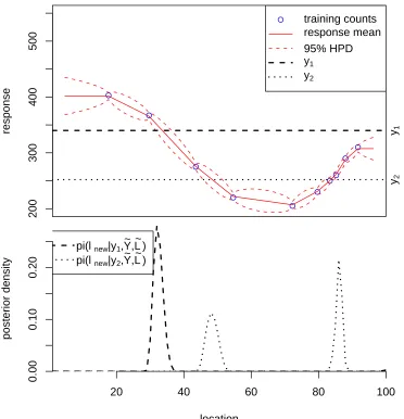
The basic idea is presented in Figure 2.2. Pollen counts ˜Y y˜j;j 1, . . . ,10on
a single plant taxon are available at 10 regularly spaced points having known climates ˜
L ˜lj. A model is fitted to these training data, represented by the smooth red line
with associated uncertainty interval (dashed red line); this is the forward stage. It models the response of a single taxon to changes in one-dimensional climate. Note that response is measured indirectly; it is a latent variable. In the context of the pollen data, response is the propensity to produce pollen, as a function of climate.
A new count ˜ynew is introduced and inferences are made on the associated
un-observed climate lnew; this is the inverse stage. The figure presents two examples
of ˜ynew. The model adopted is such that for one of these the inference on lnew is
potential mutlimodality is a consequence of the non-monotonic shape of the response surface.
The forward fitting stage is a form of non-parametric regression, in which the only requirement is that the response surface is smooth. A Bayesian approach involving a Gaussian process prior is implemented. In Section 2.5.2 a simple example is used to present the details. These are trivial if, as assumed there, the variance parameters are known and the likelihoods are Gaussian. The inverse stage, even for this toy model, is not trivial. Nevertheless, for this model, with known parameters, it is simple to compute.
This is formalised as follows, for each new count, where the Gaussian random function XL models the response surface:
πlnewSY ,˜ L,˜ y˜new
S π
lnew, XSY ,˜ y˜new,L˜dX S π
lnewSX,Y ,˜ y˜new,L˜πXSY ,˜ y˜new,L˜dX S π
lnewSX,y˜newπXSY ,˜ y˜new,L˜dX
S π
lnewSX,y˜newπXSY ,˜ L˜dX
S π
y˜newSX, lnewπlnewπXSY ,˜ L˜dX (2.24)
There are a number of interesting features of such a problem, many of which are not immediately obvious. These are most usefully demonstrated via investigation of an example toy problem, which is simple yet similar in spirit to the palaeoclimate reconstruction problem. This also serves to introduce some modelling choices which are retained throughout much of this thesis.
2.5.2
Toy Problem Example
Counts data ˜Y are available at Nd locations ˜L. The response X XL is
unob-served and treated here as a random function, defined on a fine regular grid L of
100 points across the location space. The interest here is its conditional distribution given the training data. The Bayesian formulation of the problem is then
πXSY ,˜ L˜ KπY˜SX,L˜πX K
10
M
j 1
200
300
400
500
response
training counts response mean 95% HPD
y1
y2
y1
y2
20 40 60 80 100
0.00
0.10
0.20
location
posterior density
pi(lnew|y1,Y~,L~)
pi(lnew|y2,Y
~
[image:47.612.107.479.117.503.2],L~)
whereX is the latent response andK is the normalising constant. The data are conditionally independent, given the latent surface. In such Bayesian approaches K
is source of much technical difficulty, even when πX is Gaussian. However when
the likelihood is also Gaussian, as here, Kis available analytically. For this example, the surface Xl is the likelihood mean at l>L and σ
2
Y is the variance. The prior
πXand the likelihoodπY˜SX,L˜are thus conjugate, leading to a Gaussian
poste-rior, provided the prior and likelihood precision matrices, QX and QY respectively,
are known.
Across all gridpointsL in the location space, the likelihood contributes
πYSXexp
1
2XY
TQ
YXY (2.26)
where
YL ¢ ¨ ¨ ¨ ¨ ¨ ¨ ¤ ˜
Y L L˜
0 LxL˜
(2.27)
and the likelihood precision matrixQY is diagonal and of dimensionNLNL, where
NL is the number of gridpoints. The diagonal entries are:
QY j, j ¢ ¨ ¨ ¨ ¨ ¨ ¨ ¤ 1 σ2 Y
Lj >L˜j
0 Lj ¶L˜j
(2.28)
The prior onX is an intrinsic Gaussian Markov random field (GMRF), given by
πXexp
1 2X
TQ
XX (2.29)
with the precision matrixQX given by
QX κ
1 1
1 2 1
1 2 1
1 2 1
1 2 1
The model has two scalar parameters; the positive scalar prior precision param-eter κ and the likelihood variance σ2
Y. The higher the κ value used, the greater
the smoothness of the latent surface XL. The decision to model the surface on
a regular grid rather than specifying a continuous model defined at the datapoints is due to the desirable properties of GMRFs as discussed in Section 4.1 and is not discussed here.
The Markov property is inherited by the posterior which is a multivariate Gaus-sian with mean and precision matrix given by
µ QXQY
1
QYY
Q QX QY (2.31)
Using this analytical form for the posterior of the latent surface given the data, the inverse stage posterior of Equation (2.24) may be computed numerically. The locations are discrete so the posterior for unknown location given a new count is defined only on a finite number of possible gridpoints. The posterior is therefore a probability mass function and normalisation is provided by rescaling the unnor-malised product of the prior and likelihood functions such that the total is unity. A uniform prior 1
NL is imposed here and the likelihood of the new count ˜ynew at
any given location L is NXL, σ
2
Y. The integral over the unidimensional latent
surface is performed analytically. Sample calculations are provided in Table 2.1 for a given ˜ynew.
Table 2.1: Sample calculations from the inverse stage of the toy prob-lem given a new count of 340 and the forward stage results shown in Figure 2.2.
location 28 29 30 31 32 33 34 35 36 37
prior 0.01 0.01 0.01 0.01 0.01 0.01 0.01 0.01 0.01 0.01
likelihood 3.58e9
3.95e4
9.70e3
3.22e2
4.55e2
3.90e2
2.28e2
9.32e3
2.55e3
4.16e4
product 3.58e11
3.54e6
9.70e5
3.22e4
4.55e4
3.90e4
2.28e4
9.32e5
2.46e5
4.21e6
posterior 2.20e8
2.18e3
5.96e2
1.98e1
2.80e1
2.40e1
1.40e1
5.73e2
1.51e2
2.59e3
The model parameters κ and σ2
Y effect the forward and therefore the inverse
values of κand σ2
Y are presented in Figure 2.3.
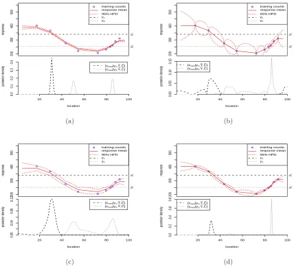
Impact of Model Parameters
Figure 2.3 illustrates the effect of varying the model parametersκandσ2
Y.
Compar-isons with the parameters used and results obtained for Figure 2.2 are made here. In Figure 2.3(a), κ is an order of magnitude larger. This induces a greater degree of smoothness in the latent surface and tightens the bounds of the 95% highest posterior density (HPD) region of the forward stage.
In Figure 2.3(b) κ is an order of magnitude smaller. The surface parameters linearly interpolate the data and uncertainty is high away from the datapoints. This leads to a highly multimodal posterior for the inverse stage. As κ goes to zero (no smoothing), the forward stage posterior tends toward the likelihood. The forward model then informs only at the datapoints and the inverse stage will yield a uniform mass function for new counts not close to training data counts. For new counts close to one or more training counts, the inverse stage posterior will be spiked at the associated training data locations.
In Figure 2.3(c)σ2
Y is an order of magnitude larger. The likelihood density has
a larger spread, as does the forward stage posterior. The prior