Estimating stellar wind parameters from low-resolution
magnetograms
M. Jardine
1 ?, A. A. Vidotto
2and V. See
11 SUPA, School of Physics & Astronomy, University of St Andrews, North Haugh, St Andrews, KY16 9SS, UK 2 School of Physics, Trinity College Dublin, The University of Dublin, Dublin-2, Ireland
Accepted XXX. Received YYY; in original form ZZZ
ABSTRACT
Stellar winds govern the angular momentum evolution of solar-like stars throughout their main-sequence lifetime. The efficiency of this process depends on the geometry of the star’s magnetic field. There has been a rapid increase recently in the number of stars for which this geometry can be determined through spectropolarimetry. We present a computationally efficient method to determine the 3D geometry of the stellar wind and to estimate the mass loss rate and angular momentum loss rate based on these observations. Using solar magnetograms as examples, we quantify the extent to which the values obtained are affected by the limited spatial resolution of stellar observations. We find that for a typical stellar surface resolution of 20o-30o, predicted
wind speeds are within 5% of the value at full resolution. Mass loss rates and angular momentum loss rates are within 5-20%. In contrast, the predicted X-ray emission measures can be under-estimated by 1-2 orders of magnitude, and their rotational modulations by 10-20%.
Key words: magnetic fields — stars: coronae — stars: winds, outflows
1 INTRODUCTION
The angular momentum evolution of solar-like stars is gov-erned by the action of their winds and in particular by the interaction between the hot, escaping gas and the stellar magnetic field (Parker 1958). Studies of these stellar winds are hampered however by the low density of the wind plasma which makes direct detection difficult (Wood et al. 2005). Of-ten the mass loss can only be inferred by studying the rota-tional distributions of samples of coeval stars in young clus-ters (Irwin et al. 2011;Delorme et al. 2011). The strength of the stellar magnetic field, which principally determines the extent of the level arm that the wind may apply, is clearly an important parameter in determine the instantaneous torque applied by the wind (Weber & Davis 1967). The field topol-ogy is also important however as only open field lines can support a wind (Mestel 1968;Mestel & Spruit 1987).
Theopenflux of magnetic field depends crucially on the geometry of the magnetic field. Over the last decade, ad-vances in spectropolarimetry have provided surface magne-tograms for a wide range of stellar masses and ages through the technique of Zeeman-Doppler imaging (Donati & Land-street 2009). These underpin theoretical efforts to model the structure and evolution of the coronae and winds of these
? E-mail: [email protected]
stars (Vidotto et al. 2009;Cranmer & Saar 2011;Matt et al. 2012; Vidotto et al. 2013; Cohen & Drake 2014; Vidotto et al. 2014a,b; Matt et al. 2015;R´eville et al. 2015b,a; Vi-dotto et al. 2015;See et al. 2015). Advances in the applica-tion of 3D MHD wind models to this data have allowed us to study the unusually powerful winds of low mass stars ( Vi-dotto et al. 2010), young active stars (Cohen et al. 2010), the role of non-potential field (Jardine et al. 2013), the impact of stellar winds on exoplanetary magnetospheres (Cohen et al. 2011;Vidotto et al. 2012) and the relationship between mass loss rates and X-ray fluxes (Vidotto et al. 2016).
Zeeman-Doppler imaging has some limitations, how-ever. It is relatively insensitive to flux in dark (spotted) regions. If this missing flux is a large contribution to the total stellar magnetic flux, its neglect may have a significant effect on the predicted X-ray emission measure ( Arzouma-nian et al. 2010; Johnstone et al. 2010). The effective sur-face resolution is also limited and while at best may be of order 5o it is typically 20o-30o. Since the polarisation
sig-nature of small-scale structures may cancel out, as much as 85%-95 % of the surface flux may be missed (Reiners & Basri 2009). A consistent picture is emerging, however, of the effect of this missing flux. By adapting solar mag-netograms,Garraffo et al.(2013) re-distributed large-scale flux onto smaller lengthscales, thus reducing the open flux, whileLang et al.(2014) artificially added a carpet of
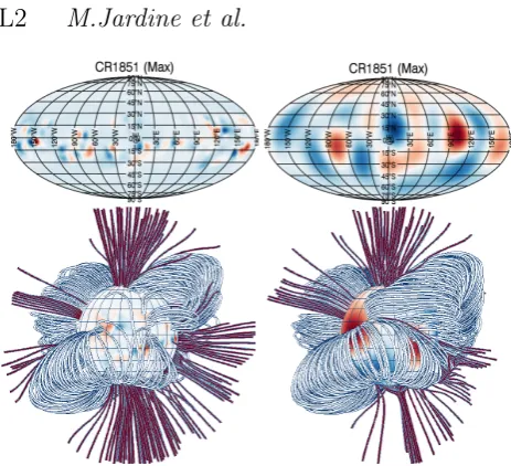
Figure 1. Top: Surface magnetograms for Carrington rotation 1851 (close to cycle maximum). The map is reconstructed for a maximum spherical harmonic degree of (left)`max = 63 and (right)`max= 5 corresponding to surface spatial scales of 3oand 30o respectively. Colourbars are set to ±200G (left) and±30G (right) . Bottom: The corresponding field extrapolations, with wind-bearing (open) field lines coloured red. The overall structure of the largest fieldlines is very similar.
scale field to Zeeman-Doppler maps of 12 M dwarfs. In the first case, the open flux was reduced, and hence the wind properties varied. In the second case, however, the open flux was unaffected. While these studies have shown the robust-ness of the stellar wind to the presence of unresolved flux, they demonstrate the much more sensitive response of the predicted X-ray emission.
As the number of stars whose surface fields has been mapped grows, so does the scope of the models of the coro-nae and winds of these stars. While fully 3D MHD models provide insight into the nature of these winds, it is clear that a more computationally efficient method of assessing the na-ture of these winds is needed. In the case of the solar wind, the availability ofin situmeasurements has made it possible to develop such an empirical wind model that is calibrated to reproduce the velocity of the solar wind at Earth. The WSA model (Wang & Sheeley 1990;Arge & Pizzo 2000) requires only the surface magnetogram as an input. The output is a fully 3D wind model, providing the local wind speed for any location within the solar wind. This model maps wind speeds directly to the degree of expansion of individual flux tubes and so is completely determined by the geometry of the magnetic field. This is typically calculated using a
Po-tential Field Source Surfacemethod that assumes the field is
[image:2.595.317.528.98.379.2]potential and is opened at some specified radius (Altschuler & Newkirk 1969). The location of this opening radius (the source surface) is a free parameter of the model that is cali-brated using solar eclipse images. Using high-resolution solar magnetogramsCohen(2015) compared this model with the output of a fully 3D MHD treatment and found differences in arrival times at Earth of more than five hours (out of a travel time of order 3 days) for only 20−40% of field lines. He also concluded that doubling the resolution of the mag-netograms from 2o to 1o has little effect on the predicted wind speeds.
Figure 2.Magnetic flux as a function of time for surface magne-tograms that have been truncated at some maximum value`max in the spherical harmonic expansion (corresponding to minimum surface spatial scales of 180o/`max). The top panel shows the sur-face flux Φsurf =H
r|Br(r)|dS, and the bottom panel shows the open flux Φopen=H
rs|Br(rs)|dS (i.e. the flux at the radius where the field becomes open).
While the WSA model has been developed for the Sun, and underlies many space weather and solar wind studies (Pinto et al. 2011; Gressl et al. 2014;Pinto et al. 2016), it has also been used in conjunction with stellar magnetograms obtained from ZDI in order to predict the impact of stel-lar winds on exoplanets (Fares et al. 2010,2012;See et al. 2014). As more exoplanets are discovered around stars with a greater range of masses and ages, there is clear demand for an efficient but reliable method of estimating wind speeds and mass loss rates of a large number of stars. In this paper, we quantify the reliability of the WSA method when used with stellar magnetograms which have a much lower resolu-tion than the solar magnetograms for which the method was developed.
2 METHOD
We take solar magnetograms obtained from the US National Solar Observatory, Kitt Peak, over two solar cycles, from February 1975 (CR1625) to April 2000 (CR1962). Fig. 1
shows one example, taken from close to solar maximum. Since the surface field can be expressed as a sum of spherical harmonics, it is possible to truncate this sum at any order of the expansion. A magnetogram where a maximum order
`maxhas been used therefore corresponds to a minimum
spa-tial scale at the stellar surface of 180o/`
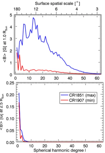
Figure 3.Mean flux density< B >at each individual`degree in the spherical harmonic expansion (corresponding to surface spatial scales of 180o/`). This is defined as < B >= Φ/4πr2 where the flux through some radiusr is Φ =H
r|Br|dS. In the top panel, this surface isr=r, whereas in the bottom panel we
choose the start of the wind-bearing regionr=rs.
the field using the Potential Field Source Surface method, with a source surface at 2.5r(Riley et al. 2006).
2.1 Modelling the magnetic field
We assume that the field is potential and divergence-free, such that ifB =−∇ψ, thenψ satisfies Laplace’s equation
∇2
ψ= 0 with solution in spherical co-ordinates (r, θ, φ)
Br= N
X
l=1 l
X
m=−l
[lalmrl
−1−
(l+ 1)blmr
−(l+2)
]Plm(cosθ)eimφ
(1)
Bθ=− N
X
l=1 l
X
m=−l
[almrl−1−blmr−(l+2)]
d
dθPlm(cosθ)e
imφ
(2)
Bφ=− N
X
l=1 l
X
m=−l
[almrl−1−blmr−(l+2)]
Plm(cosθ)
sinθ ime
imφ
(3)
Figure 4.Variation with maximum spherical harmonic degree `max of the average wind speed at the Earth’s orbit, the total mass loss rate and the total angular momentum loss rate.
where all radii are scaled to a stellar radius and the associ-ated Legendre polynomials are denoted byPlm. The two
un-knowns are the coefficientsalmandblm. One of these can be
determined by imposing the radial field at the surface from the Zeeman-Doppler maps. The second is determined by im-posing the condition that at the source surface (r=rs), the
field is purely radial, such thatBθ(rs) =Bφ(rs) = 0. We use
a code originally developed byvan Ballegooijen et al.(1998) (see alsoJardine et al.(2002)).
Fig.2shows the surface flux and the open flux for maps sampled at different`max values. Fig.3 shows, for two
ex-ample magnetograms (one close to solar maximum and the other close to solar minimum), the distribution of power in the magnetic field at different lengthscales. The top panel shows that when the Sun is at its most active, the peak power is around`max= 13, ie the scale size of the magnetic
[image:3.595.323.525.103.528.2] [image:3.595.42.284.608.779.2]also Vidotto (2016)). At higher `-values, there is progres-sively less power. When the Sun is inactive, the peak power is in the dipole term and there is little power beyond`max= 5.
The bottom panel shows that in the wind-dominated regime, only the lowest-order modes survive.
2.2 Modelling the wind
For each field line (labelledi) the velocityuialong that field
line at the Earth’s orbit is given by (Wang & Sheeley(1990);
Arge & Pizzo(2000))
ui[kms
−1
] = 267.5 +410.0
fi2/5 (4)
where the expansion factorfi of any field line is given by:
fi=
r2
r2 s
Bi(r)
Bi(rs)
. (5)
We assume that the magnetic field expands radially beyond the source surface and determine the mass loss rate from a 1D isothermal wind solution along each field line. The requirement that the wind is trans-sonic and reaches the velocity ui at Earth then determines the field line
temper-ature. We assume that the plasma pressure at the base of the field line is given by p0 =κwB20 where we set the free
parameterκw to a value that produces the variation in the
solar mass loss rate through its cycle (Cranmer 2008). Com-bined with the temperature, this base pressure determines the base density. Conservation of mass and magnetic flux re-quires thatρu/Bis constant along each flux tube, providing the mass loss rate through a spherical surface at the Earth’s orbit (SE)
˙
M =
I
SE
ρiuidSi (6)
where ρi is the density at the Earth’s orbit and dSi is
the cross-sectional area of the flux tube. Along each field line the Alfv´en radius is then the location where u(r) =
B(r)/pµρ(r). From this, we can estimate the total angular momentum loss rate by integrating over the Alfv´en surface (SA)
˙
J=
I
SA
ρ(u·n)Ω?$2dSA (7)
where n is the outward normal, Ω? is the stellar angular
velocity and $ is the cylindrical radius. We note that this neglects the small term due to non-axisymmetry described inMestel(1999). Fig.4shows the effect of the surface resolu-tion on the predicted wind speed, mass loss rate and angular momentum loss rate.
2.3 Modelling the X-ray emission measure
We model the X-ray emission measure by assuming that the gas on each closed field line is in hydrostatic, isother-mal equilibrium. The gas pressure is therefore p =
p0e m kT
R
gsds where g
s = (g.B)/|B| is the component of
gravity (allowing for rotation) along the field andg(r, θ) =
−GM?/r2+ Ω2?rsin2θ,Ω2?rsinθcosθ
. The plasma pres-sure at the base of each field linep0=κcB02 where the free
parameterκcis fixed by the overall stellar X-ray luminosity.
[image:4.595.323.521.100.263.2]In order to quantify the effect of changing the resolution of
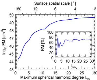
Figure 5.Variation with maximum spherical harmonic degree of the emission measure for CR1851 at 106K. The inset shows the rotational modulation RM = (EMmax−EMmin)/EMmax.
the surface magnetogram, we select the example in Fig.1. Fig.5shows the resulting emission measures that correspond to a temperature of 106K, and their rotational modulations.
3 RESULTS AND DISCUSSION
By decomposing solar magnetograms into spherical harmon-ics which can be truncated at different orders, we have shown the variation over the solar cycle of the various contributions to the Sun’s magnetic field. As also found byDeRosa et al.
(2012), Fig.2shows that the dipole mode has a cyclic vari-ation that is in antiphase with the higher order modes. At each time we can also analyse the distribution of power in the magnetic field at various lengthscales (or spherical har-monic orders). At cycle maximum, this power peaks at an spherical harmonic degree determined by the spatial scale on which magnetic bipoles appear on the surface. At cy-cle minimum in contrast, only the lowest-order (ie largest length scale) modes contribute (Vidotto 2016). By extrapo-lating this surface field out into the corona, we find that only the lowest-order modes persist out to the height at which the wind dominates over the closed corona. The flux ofopen
magnetic field is therefore sensitive only to the lowest or-der modes and therefore the largest lengthscale variations of the surface field. This behaviour alone suggests that the behaviour of the stellar wind (its speed, mass loss rate and angular momentum loss rate) can be well approximated by the information in low-resolution stellar magnetograms.
To quantify this effect, we select as an example the WSA model that predicts the 3D distribution of the solar wind speed at the Earth’s orbit. We determine the variation of this wind speed with the resolution of the surface magnetogram and find that for a typical stellar surface resolution of 20o -30o, typical predicted wind speeds are within 5% of the value
at full resolution. Mass loss rates and angular momentum loss rates are typically within 5-20%.
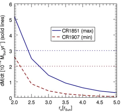
Figure 6. Variation with source surface radius rs of the mass loss rate M˙. Dotted horizontal lines show the average values at solar maximum and minimum (Cranmer 2008). An increase in rs from 2.2-2.7 r between these two Carrington rotations
would reproduce the observed values at these times of around 2×10⁻¹⁴M
yr−1.
of surface activity as the Sun, we might underestimate the emission measure by 1-2 orders of magnitude. The rotational modulation is also affected, varying from zero (the aligned dipole at solar minimum) to 80% at full resolution.
Our studies therefore suggest that wind speeds, mass, and angular momentum loss rates are insensitive to the loss of information produced by the low surface resolution of stel-lar magnetograms. These calculations, however, involve two free parameters - the source surface radius rs and the
con-stant κw. The mass loss rate scales linearly with κw. We
have selected a value that reproduces the observed range of solar mass loss rates (Cranmer 2008). Fig.6shows the effect of varying the other free parameterrs. The observed range
could be reproduced with only modest adjustments ofrs.
Extending this method to other stars for which surface magnetograms are available clearly requires some assump-tions about the behaviour of rs and κ. Following Mestel & Spruit (1987) we suggest fixing both to the values used here for the Sun, allowing the surface magnetograms (which determine B0) in addition to the stellar mass, radius and
rotation rate, to govern the predicted wind properties. This produces mass loss rates for solar-like stars that compare well with those determined from fully 3D MHD wind mod-els (See et al, 2017, submitted).
ACKNOWLEDGEMENTS
The authors acknowledge support from STFC.
REFERENCES
Altschuler M. D., Newkirk G., 1969,Sol. Phys.,9, 131 Arge C. N., Pizzo V. J., 2000,J. Geophys. Res.,105, 10465 Arzoumanian D., Jardine M., Donati J., Morin J., Johnstone C.,
2010, preprint, (arXiv:1008.3613) Cohen O., 2015,Sol. Phys.,290, 2245
Cohen O., Drake J. J., 2014,ApJ,783, 55
Cohen O., Drake J. J., Kashyap V. L., Hussain G. A. J., Gombosi T. I., 2010,ApJ,721, 80
Cohen O., Kashyap V. L., Drake J. J., Sokolov I. V., Garraffo C., Gombosi T. I., 2011,ApJ,733, 67
Cranmer S. R., 2008, in van Belle G., ed., Astronomical Soci-ety of the Pacific Conference Series Vol. 384, 14th Cambridge Workshop on Cool Stars, Stellar Systems, and the Sun. p. 317 (arXiv:astro-ph/0701561)
Cranmer S. R., Saar S. H., 2011,ApJ,741, 54
DeRosa M. L., Brun A. S., Hoeksema J. T., 2012,ApJ,757, 96 Delorme P., Collier Cameron A., Hebb L., Rostron J., Lister T. A.,
Norton A. J., Pollacco D., West R. G., 2011,MNRAS,413, 2218
Donati J.-F., Landstreet J. D., 2009,ARA&A,47, 333 Fares R., et al., 2010,MNRAS,406, 409
Fares R., et al., 2012,MNRAS,423, 1006
Garraffo C., Cohen O., Drake J. J., Downs C., 2013,ApJ,764, 32 Gressl C., Veronig A. M., Temmer M., Odstrˇcil D., Linker J. A.,
Miki´c Z., Riley P., 2014,Sol. Phys.,289, 1783
Irwin J., Berta Z. K., Burke C. J., Charbonneau D., Nutzman P., West A. A., Falco E. E., 2011,ApJ,727, 56
Jardine M., Collier Cameron A., Donati J.-F., 2002, MNRAS, 333, 339
Jardine M., Vidotto A. A., van Ballegooijen A., Donati J.-F., Morin J., Fares R., Gombosi T. I., 2013,MNRAS,431, 528 Johnstone C., Jardine M., Mackay D. H., 2010,mnras,404, 101 Lang P., Jardine M., Morin J., Donati J.-F., Jeffers S., Vidotto
A. A., Fares R., 2014,MNRAS,439, 2122
Matt S. P., MacGregor K. B., Pinsonneault M. H., Greene T. P., 2012,ApJ,754, L26
Matt S. P., Brun A. S., Baraffe I., Bouvier J., Chabrier G., 2015, ApJ,799, L23
Mestel L., 1968, MNRAS, 138, 359 Mestel L., 1999, Stellar magnetism
Mestel L., Spruit H. C., 1987, MNRAS, 226, 57 Parker E., 1958, ApJ, 128, 664
Pinto R. F., Brun A. S., Jouve L., Grappin R., 2011,ApJ,737, 72
Pinto R. F., Brun A. S., Rouillard A. P., 2016,A&A,592, A65 Reiners A., Basri G., 2009,A&A,496, 787
R´eville V., Brun A. S., Matt S. P., Strugarek A., Pinto R. F., 2015a,ApJ,798, 116
R´eville V., Brun A. S., Strugarek A., Matt S. P., Bouvier J., Folsom C. P., Petit P., 2015b,ApJ,814, 99
Riley P., Linker J. A., Miki´c Z., Lionello R., Ledvina S. A., Luh-mann J. G., 2006,ApJ,653, 1510
See V., Jardine M., Vidotto A. A., Petit P., Marsden S. C., Jeffers S. V., do Nascimento J. D., 2014,A&A,570, A99
See V., et al., 2015, MNRAS
Vidotto A. A., 2016,MNRAS,459, 1533
Vidotto A. A., Opher M., Jatenco-Pereira V., Gombosi T. I., 2009, ApJ,699, 441
Vidotto A., Jardine M., Opher M., Donati J.-F., Gombosi T. I., 2010, MNRAS
Vidotto A. A., Fares R., Jardine M., Donati J.-F., Opher M., Moutou C., Catala C., Gombosi T. I., 2012, MNRAS,423, 3285
Vidotto A. A., Jardine M., Morin J., Donati J.-F., Lang P., Rus-sell A. J. B., 2013,A&A,557, A67
Vidotto A. A., Jardine M., Morin J., Donati J. F., Opher M., Gombosi T. I., 2014a,MNRAS,438, 1162
Vidotto A. A., et al., 2014b,MNRAS,441, 2361
Vidotto A. A., Fares R., Jardine M., Moutou C., Donati J.-F., 2015,MNRAS,449, 4117
Wood B. E., M¨uller H.-R., Zank G. P., Linsky J. L., Redfield S., 2005,apjl,628, L143
van Ballegooijen A., Cartledge N., Priest E., 1998, ApJ, 501, 866