Block Method for Solving Pantograph-type Functional Differential Equations

(1)



Abstract— In this paper, we describe the development of a two-point block method for solving pantograph-type functional differential equations. The block method, implemented in variable stepsize technique produces two approximations simultaneously using the same back values. The grid-point formulae for the variable steps are derived, calculated and stored at the start of the program for greater efficiency. The delay solutions for the unknown function and its derivative at earlier times are interpolated using the previous computed values. Stability regions for the block method are illustrated. Numerical results are given to demonstrate the accuracy and efficiency of the block method.

Index Terms—Block method, functional differential equation, pantograph equation, polynomial interpolation, stability region

I. INTRODUCTION

UNCTIONAL differential equation of the form

))) ( ( )), ( ( ), ( , ( )

(x f x y x y x y x

y    (1)

appears in many real life applications and has been investigated by many authors in recent years. The classical case is when (x)x. When the right hand side of (1) does not depend on the derivative of the unknown function y, the equation is known as delay differential equation. Otherwise, it is known as neutral delay differential equation.

In this paper, we consider numerical solution for functional differential equation of the form:

  



  

 

, ) 0 (

, 0 )), ( ), ( ), ( , ( ) (

0 y y

T x qx

y qx y x y x f x y

(2) where 0q1. Equation (2), known as the pantograph equation arises in many physical applications such as number theory, electrodynamics, astrophysics, etc.. Detailed explanations can be found in [1] – [3]. Numerical solutions for (2) have been studied extensively, see for example [4] –

Manuscript received March 01, 2013; revised April 02, 2013. This work was supported in part by Universiti Teknologi MARA and the Ministry of Higher Education of Malaysia (MOHE) under the Fundamental Research Grant Scheme (FRGS) 600-RMI/ST/FRGS 5/3/Fst (20/2011).

F. Ishak is with the Faculty of Computer and Mathematical Sciences, Universiti Teknologi MARA, 40450 Shah Alam, Selangor, MALAYSIA (phone: +603-5543-5348; fax: +603-543-5501; e-mail: fuziyah@ tmsk.uitm.edu.my).

M. B. Suleiman is with the Institute for Mathematical Research (INSPEM), Universiti Putra Malaysia, 43400 Serdang, MALAYSIA (e-mail: [email protected]).

Z. A. Majid is with the Mathematics Department, Universiti Putra Malaysia, 43400 Serdang, MALAYSIA (e-mail: [email protected]).

[7] and the references cited therein. These methods produce one approximation in a single integration step. Block methods, however produce more than one approximation in a step. Block methods have been used to solve wide range of ordinary differential equations as well as delay differential equations (see [8] – [11] and the references cited therein).

In this paper, we solve (2) using a two-point block method in variable step. In a single integration step, two new approximates for the function y in (2) are obtained while keeping a constant stepsize, doubling or halving. The coefficients of the method need to be recalculate whenever the stepsize changes. In order to avoid the tedious calculation, the coefficients based on the stepsize ratio are calculated beforehand and stored at the start of the program. The organization of this paper is as follows. In section II, we briefly describe the development of the variable step block method. Stability region for the block method is discussed in section III. Numerical results for some pantograph equations are presented in section IV and finally section V is the conclusion.

II. METHOD DEVELOPMENT

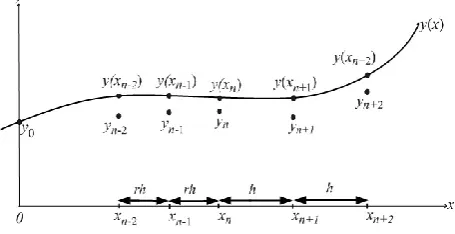
Referring to (2), we seek a set of discrete solutions for the unknown function y in the interval [0,T]. The interval is divided into a sequence of mesh points

 

x_i t_i_₀ of different lengths, such that 0x₀ x₁x_t T.Let the approximated solution for y(x_n)be denoted as y_n. Suppose that the solutions have been obtained up to x_n. At the current step, two new solutions y_n_₁ and y_n_₂ at x_n_₁ and

2 

n

[image:1.595.318.546.653.770.2]

x respectively are simultaneously approximated using the same back values by taking the same stepsize. The points xn1 and xn2 are contained in the current block. The length of the current block is 2h. We refer to this particular block method as two-point one-block method. The block method is shown in Fig 1.

Fig 1. Two-point one-block method

Block Method for Solving Pantograph-type

Functional Differential Equations

Fuziyah Ishak, Mohamed B. Suleiman, and Zanariah A. Majid

(2)

In Fig 1, the stepsize of the previous step is viewed in the multiple of the current stepsize. Thus, x_n_₁x_nh,

h x

x_n_₂ _n_₁ and x_n_₁x_n_₂x_nx_n_₁rh. The value of r is either 1, 2, or

2

1 _{, depending upon the decision to} change the stepsize. In this algorithm, we employ the strategy of having the stepsize to be constant, halved or doubled.

The formulae for the block method can be written as the pair, ), ˆ , , , ( ) ( ), ˆ , , , ( ) ( 2 2 2 2 4 0 * 2 2 2 2 2 4 0 1 i n i n i n i n i i n n i n i n i n i n i i n n y y y x f r h y y y y y x f r h y y                    



      (3)

where y_n and yˆ_n are the approximations to y(qx_n) and )

(qxn

y respectively. For simplicity, from now on we refer to f(x_n,y_n,y_n,yˆ_n)as f_n. The coefficient functions _i(r) and



i*(r) will give the coefficients of the method when r is either 1, 2, or

2 1 _.

The first formula in (3) is obtained by integrating (2) from

n

x to x_n_₁ while replacing the function f with the polynomial Pwhere P(x)is given by

, ) ( ) ( 4 0 2 , 4



    j j n j x f

L x P and . 4 , , 1 , 0 for , ) ( ) ( ) ( 4

0 2 2

2 ,

4 _  

 



       _j x x x x x L j i

i n j n i i n j

Similarly, the second formula in (3) is obtained by integrating (2) from xn to xn2 while replacing the function f with the polynomial P. The value of y_n is obtained by the interpolation function such as,

], , , [ ) ( ) ( ] , [ ) ( ] [ 4 3 1           j j j n j n j j j n j n x x y x qx x qx x x y x qx x y y    where , ] , , [ ] , , [ ] , , , [ 4 4 1 3 4 1       _   j j j j j j j j

j _x _x

x x y x x y x x x

y   

provided that xj₁qxnxj, n j, j1. We approximate the value of yˆ_n by interpolating the values of

f , that is,

], , , [ ) ( ) ( ] , [ ) ( ] [ ˆ 4 3 1           j j j n j n j j j n j n x x f x qx x qx x x f x qx x f y    where . ] , , [ ] , , [ ] , , , [ 4 4 1 3 4 1       _   j j j j j j j j

j _x _x

x x f x x f x x x

f   

The formulae in (3) are implicit, thus a set of predictors are derived similarly using the same number of back values.

For greater efficiency while achieving the required accuracy, the algorithm is implemented in variable stepsize scheme. The stepsize is changed based on the local error that is controlled at the second point. A step is considered successful if the local error is less than a specified tolerance. If the current step is successful, we consider either doubling or keeping the same stepsize. If the same stepsize had been used for at least two blocks, we double the next stepsize. Otherwise, the next stepsize is kept the same. If the current step fails, the next stepsize is reduced by half. For repeated failures, a restart with the most optimal stepsize with one back value is required. For variable step algorithms, the coefficients of the methods need to be recalculated whenever a stepsize changes. The recalculation cost of these coefficients is avoided by calculating the coefficients beforehand and storing them at the start of the program. With our stepsize changing strategy, we store the coefficients _i(r) and *(_r)

i



for ris 1, 2 and . 2 1

III. REGION OF ABSOLUTE STABILITY

In the development of a numerical method, it is of practical importance to study the behavior of the global error. The numerical solution y_n is expected to behave as the exact solution y(x_n)does as x_napproaches infinity. In this section, we present the result of stability analysis of the two-point one-block method when they are applied to the neutral delay differential equations with real coefficients.

For the sake of simplicity and without the lost of generality, we consider the equation

, 0 ), ( ) ( , 0 ), ( ) ( ) ( ) (             x x x y x x y c x by x ay x y     (4) where a,b,cR,  is the delay term such as



mh, his a constant stepsize such that x_nx₀nh and mZ. If

, 

Z

i we define vectors _

           i n i n i N _y y 2 2 2 3

Y and

. 2 2 2 3             i n i n i N _f f

F Then, the block method (3) can be written in matrix form such as,

, ) ( 2 0 2 2 1 1



      i i N i N

N A h B r

AY Y F (5)

where ,

1 0 1 0 1          A , 1 0 0 1 2       

A and B_i(r) is a matrix that contains the coefficients _i(r) and



i*(r). Applying method (5) to (4), we get

, ) ( ) ( 1 1 2 2 2 0 2 0 2 1 2 2 1 1 m N m N i i m i N i i N i N N cA cA r B H r B H A A                



Y Y Y Y Y Y

where H₁ha and H₂ hb. Rearranging, we have , ) ) ( ( )) ( ( 2 0 2 2 0 1



        i m i N i i i i N i

i H B r H B r cA

A Y Y (6)

(3)

(6) is given by C_m(H₁,H₂,c;) where C_m is the determinant of . 0 ) ) ( ( )) ( ( 2 0 2 2 0

1   





   i i i i i i m i

i H B r H B r cA

A   (7)

The numerical solution (6) is asymptotically stable if and only if for all m,all zeros of the characteristic polynomial (7) lie within the open unit disk in the plane. The stability region is defined as follows:

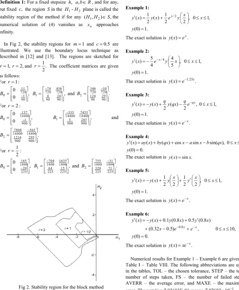
Definition 1: For a fixed stepsize ,h a,bR, and for any, but fixed c, the region Sin the H₁-H₂ plane is called the stability region of the method if for any (H₁,H₂)S,the numerical solution of (4) vanishes as x_n approaches infinity.

In Fig 2, the stability regions for m1 and c0.5 are illustrated. We use the boundary locus technique as described in [12] and [13]. The regions are sketched for

, 1



r r2,and . 2 1



r The coefficient matrices are given as follows:

For r1: , 0 0 901 72011 0          _ B , 90 24 904 720 456 72074 1          

B and .

90 29 90 124 720 10 720 346 2           B

For r2: , 0 0 9001 14400137 0          _ B , 900285 9005 144007455 14400335 1           B and . 900 295 900 1216 14400 565 144007808 2           B

For :

2 1  r , 0 0 22520 1800145 0          _ B , 22515 22564 1800 1635 1800704 1          

B and .

[image:3.595.49.536.180.771.2]

22571 225 320 1800 31 1800755 2           B

Fig 2. Stability region for the block method

Referring to Fig 2, the stability regions are closed region bounded by the corresponding boundary curves. It is observed that the stability region shrinks as the stepsize increases.

IV. NUMERICAL RESULTS

In this section, we present some numerical examples in order to illustrate the accuracy and efficiency of the block method. The examples taken and cited from [7] are as follows: Example 1: . 1 ) 0 ( , 1 0 , 2 2 1 ) ( 2 1 )

( /2

            y x x y e x y x y x

The exact solution is y(x)ex. Example 2: . 1 ) 0 ( , 1 0 , 5 4 4 5 )

( /4

             y x x y e x y x

The exact solution is y(x)e1.25x. Example 3: . 1 ) 0 ( , 1 0 , 2 ) ( 2 ) ( ) (          y x e q qx y q x y x y qx

The exact solution is y(x)ex. Example 4: . 0 ) 0 ( , 1 0 ), sin( sin cos ) ( ) ( ) (          y x qx b x a x qx by x ay x y

The exact solution is y(x)sinx. Example 5: . 1 ) 0 ( , 1 0 , 2 2 1 2 2 1 ) ( ) (                      y x x y x y x y x y

The exact solution is y(x)ex. Example 6: . 0 ) 0 ( , 10 0 , ) 5 . 0 32 . 0 ( ) 8 . 0 ( 5 . 0 ) 8 . 0 ( 1 . 0 ) ( ) ( 8 . 0               y x e e x x y x y x y x y x x

The exact solution is _y(_x)__xex.

(4)

[image:4.595.56.296.67.164.2]

Table I: Numerical Results for Example 1

TOL STEP FS AVERR MAXE

2

10 20 0 7.02683E-01 9.68012E-05 4

10 27 0 4.15905E-07 9.05425E-07 6

10 35 0 3.09498E-07 4.21310E-07 8

10 48 0 9.55941E-09 1.28084E-08 10

[image:4.595.312.557.92.192.2]

10 75 0 7.68855E-11 9.88663E-11

Table II: Numerical Results for Example 2

2

10 21 0 9.76063E-08 1.17093E-07 4

10 27 0 4.95202E-09 1.27731E-07 6

10 35 0 1.06955E-09 1.21167E-08 8

10 50 0 3.12606E-11 1.43148E-10 10

[image:4.595.56.295.215.314.2]

10 79 0 5.60297E-13 1.51457E-12

Table III: Numerical Results for Example 3, q0.2

2

10 20 0 1.54360E-05 1.91824E-05 4

10 27 0 1.15315E-07 5.14934E-07 6

10 35 0 6.83967E-08 8.52745E-08 8

10 47 0 2.03160E-09 2.57931E-09 10

10 74 0 1.50180E-11 2.00260E-11

Table IV: Numerical Results for Example 3, q0.8

2

10 20 0 1.57507E-07 2.30455E-06 4

10 27 0 2.90818E-08 4.90683E-07 6

10 35 0 4.03006E-10 3.90288E-09 8

10 48 0 2.46267E-11 1.51318E-10 10

10 74 0 3.09422E-13 1.74260E-12

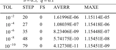
Table V: Numerical Results for Example 4, a1, b0.5, q0.1

2

10 20 0 1.61996E-06 1.15114E-05 4

10 27 0 1.08039E-07 1.15418E-06 6

10 35 0 8.23406E-09 1.15448E-07 8

10 48 0 5.74175E-10 1.15451E-08 10

[image:4.595.313.554.243.341.2]

10 79 0 4.12730E-11 1.15451E-09

Table VI: Numerical Results for Example 4, a1, b0.5, q0.5

2

10 20 0 6.25587E-06 4.77895E-05 4

10 27 0 4.53165E-07 4.78257E-06 6

10 35 0 3.48942E-08 4.78294E-07 8

10 50 0 2.91205E-09 4.78298E-08 10

[image:4.595.54.297.367.464.2]

10 79 0 1.83823E-10 4.78299E-09

Table VII: Numerical Results for Example 5

2

10 20 0 7.31358E-04 1.83509E-03 4

10 27 0 1.88577E-05 2.92294E-05 6

10 71 0 9.02824E-06 2.12659E-05 8

10 166 2 1.14939E-06 2.13569E-06 10

10 236 4 4.56047E-08 5.25142E-08

Table VIII: Numerical Results for Example 6

2

10 70 0 1.22749E-02 4.54860E-02 4

10 97 0 3.92866E-04 1.14032E-03 6

10 118 0 1.61615E-06 4.86641E-06 8

10 173 0 2.72657E-07 4.87304E-07 10

10 300 3 1.72160E-08 3.97650E-08

From Table 1 – Table VIII, it is observed that for the given tolerances, the two-point block method achieves the desired accuracy. When the tolerance becomes smaller, the total number of steps increases. In order to achieve the desired accuracy, smaller stepsizes are taken, thus resulting in the increase number of total steps taken.

V. CONCLUSION

[image:4.595.312.555.391.488.2] [image:4.595.56.295.519.615.2] [image:4.595.55.295.669.774.2]

(5)

REFERENCES

[1] R. D. Driver, Ordinary and Delay Differential Equations, New York: Springer-Verlag, 1977.

[2] J. R. Ockendon and A. B. Taylor, “The dynamics of a current collection system for an electric locomotive,” Proc. R. Soc. Lond., Ser. A 322, pp. 447–468, 1971.

[3] A. Iserles, “On the generalized pantograph functional differential equation,” European Journal of Appl. Math, vol. 4, pp. 1–38, 1992. [4] D. J. Evans and K. R. Raslan, “The Adomian decomposition method

for solving delay differential equation,” International Journal of

Computer Mathematics, vol. 82, no. 1, pp. 49–54, 2005.

[5] W. S. Wang and S. F. Li, “On the one-leg -methods for solving nonlinear neutral functional differential equations,” Applied

Mathematics and Computation, vol. 193, pp. 285–301, 2007.

[6] I. Ali, H. Brunner and T. Tang, “A spectral method pantograph-type delay differential equations and its convergence analysis ,” Journal of

Computational Mathematics, vol. 27, no. 2-3, pp. 254–265, 2009.

[7] S. Sedaghat, Y. Ordokhani and M. Dehghan, “Numerical solution of the delay differential equations of pantograph type via Chebyshev polynomials,” Commun Nonlinear Sci Numer Simulat, vol.137, pp. 4815–4830, 2012.

[8] Z. A. Majid, “Parallel block methods for solving ordinary differential equations,” Ph.D. thesis, Universiti Putra Malaysia., 2004.

[9] F. Ishak, M. Suleiman and Z. Omar, “Two-point predictor-corrector block method for solving delay differential equations” Matematika, vol.24, no. 2, pp. 131–140, 2008.

[10] F. Ishak, Z. A. Majid and M. Suleiman, “Two-point block method in variable stepsize technique for solving delay differential equations ”

J. of Materials Sc. and Engineering, vol.4, no. 12, pp. 86–90, 2010.

[11] F. Ishak, Z. A. Majid and M. B. Suleiman, “Development of implicit block method for solving delay differential equations,” in Proc. 14th WSEAS Int. Conf on Mathematical and Comp. Methods in Sc. and

Engineering, Malta, 2012, pp. 67–71.

[12] C. T. H. Baker and C. A. H. Paul, “Computing stability regions-Runge-Kutta methods for delay differential equations ” IMA Journal

of Num. Analysis, vol.14, pp. 347–362, 1994.