Open Access
Software
Biochemical Network Stochastic Simulator (BioNetS): software for
stochastic modeling of biochemical networks
David Adalsteinsson*
1, David McMillen
2and Timothy C Elston
1Address: 1Department of Mathematics, University of North Carolina at Chapel Hill, Chapel Hill, NC 27599-3250, USA and 2Department of
Chemical and Physical Sciences, University of Toronto at Mississauga, Mississauga, ON L5L 1C6, Canada Email: David Adalsteinsson* - [email protected]; David McMillen - [email protected]; Timothy C Elston - [email protected]
* Corresponding author
Abstract
Background: Intrinsic fluctuations due to the stochastic nature of biochemical reactions can have large effects on the response of biochemical networks. This is particularly true for pathways that involve transcriptional regulation, where generally there are two copies of each gene and the number of messenger RNA (mRNA) molecules can be small. Therefore, there is a need for computational tools for developing and investigating stochastic models of biochemical networks.
Results: We have developed the software package Biochemical Network Stochastic Simulator (BioNetS) for efficiently and accurately simulating stochastic models of biochemical networks. BioNetS has a graphical user interface that allows models to be entered in a straightforward manner, and allows the user to specify the type of random variable (discrete or continuous) for each chemical species in the network. The discrete variables are simulated using an efficient implementation of the Gillespie algorithm. For the continuous random variables, BioNetS constructs and numerically solves the appropriate chemical Langevin equations. The software package has been developed to scale efficiently with network size, thereby allowing large systems to be studied. BioNetS runs as a BioSpice agent and can be downloaded from http://www.biospice.org. BioNetS also can be run as a stand alone package. All the required files are accessible from http://x.amath.unc.edu/BioNetS.
Conclusions: We have developed BioNetS to be a reliable tool for studying the stochastic dynamics of large biochemical networks. Important features of BioNetS are its ability to handle hybrid models that consist of both continuous and discrete random variables and its ability to model cell growth and division. We have verified the accuracy and efficiency of the numerical methods by considering several test systems.
Background
Mathematical modeling of complex biological networks has a lengthy history [1-5]. In the past, the standard approach for modeling these systems has been to derive ordinary differential equations (ODEs) based on the law of mass action for the concentrations of the biochemical species involved in the network [6-16]. Experimental studies [17-19] have demonstrated, however, that
sto-chastic effects can be significant in cellular reactions, par-ticularly in the case of transcriptional regulation, where generally there are two copies of each gene and the number of messenger RNA (mRNA) molecules can be small. A number of recent experimental and modeling studies have addressed the role of fluctuations in gene expression [20-31]. Many modeling studies have employed the well-established Gillespie Monte Carlo
Published: 08 March 2004 BMC Bioinformatics 2004, 5:24
Received: 07 November 2003 Accepted: 08 March 2004 This article is available from: http://www.biomedcentral.com/1471-2105/5/24
© 2004 Adalsteinsson et al; licensee BioMed Central Ltd. This is an Open Access article: verbatim copying and redistribution of this article are permitted in all media for any purpose, provided this notice is preserved along with the article's original URL.
algorithm [32] or one of its more recent variants [33,34]. These algorithms offer an exact solution to the stochastic evolution of chemical systems, but they are computation-ally very expensive. A much more efficient approach is to approximate the species as continuous variables and for-mulate the problem in terms of stochastic differential equations (SDEs), often referred to as chemical Langevin equations [24,28,35]. This approximation works remark-ably well for many cases, even when the number of parti-cles involved is as small as ten, and the resulting simulations can run orders of magnitude more quickly than the discrete Monte Carlo approach. In other cases, when some or all of the particle numbers are very small, the system may need to be modeled using the discrete approach, or a hybrid method in which some species are treated discretely while others are evolved using the con-tinuum approximation. With the increasing interest in formulating accurate models of large biochemical net-works, there is a need for reliable software packages that correctly incorporate stochastic effects, yet are fast enough to simulate large interconnected sets of reacting species (as found, for example, in signaling cascades or genetic regulatory networks). We have developed the BIOchemi-cal NETwork Stochastic Simulator, "BioNetS," to meet this need. BioNetS is capable of performing full discrete simu-lations using an efficient implementation of the Gillespie algorithm. It is also able to set up and solve the chemical Langevin equations, which are a good approximation to the discrete dynamics in the limit of large abundances. Finally, BioNetS can handle hybrid models in which chemical species that are present in low abundances are treated discretely, whereas those present at high abun-dances are handled continuously. Thus, the user can pick the simulation method that is best suited to their needs. All aspects of the software are highly optimized for efficiency.
The remainder of this manuscript is arranged in the fol-lowing way. In the Implementation section, the mathe-matical background for the Gillespie method, chemical Langevin equations and hybrid models is presented, along with a discussion of the numerical algorithms used in BioNetS. Under Results and Discussion we provide a brief introduction to BioNetS along with several exam-ples. The examples serve two purposes: 1) to illustrate how to use the software and 2) to verify its efficiency and accuracy. More complete documentation can be found at http://x.amath.unc.edu/BioNetS, and in the documenta-tion included with the package.
Implementation
We first develop the mathematical methodology on which BioNetS is built. Readers interested in using Bio-NetS without going into its underlying structure can pro-ceed directly to the Results and discussion section.
Discrete reactions and the gillespie algorithm
BioNetS makes use of elementary reactions (zeroth, first and second order). The following examples illustrates each type of reaction:
In the above reactions, the calligraphic letters denote a single molecule of a chemical species. The number of mol-ecules of a particular species in the system at time t is denoted with uppercase letters (e.g., A(t), B(t), A_B(t), and V(t)). All the rate constants, γ, δ, and k1-k6, have units of per time. Eq. 1 represents a process in which a molecule
A is produced when the reaction proceeds in the forward
direction and is degraded in the reverse direction. In the forward direction the reaction is zeroth order and pro-ceeds with an average rate of γ. In the backward direction, the reaction is first order, and the average rate of degradation is δA(t). The forward reaction in Eq. 2 repre-sents a process in which chemical species A is converted to species B. In this case A and B might represent two differ-ent conformations of the same molecule. In Eq. 2 both the forward and backward reactions are first order because the reaction rates are proportional to the respective concentra-tions. The forward reaction given in Eq. 3 is a second order reaction in which an A molecule and a B molecule come together to form the complex A_B. The average rate for the reaction is k1A(t)B(t). The backward reaction is a first
order reaction in which A_B dissociates at an average rate of k2A_B(t). In Eq. 4 the forward reaction produces a
mol-ecule V. The difference between this reaction and the for-ward reaction in Eq. 1 is that the average rate is k3V(t). This
leads to exponential growth of V(t). This reaction is par-ticularly useful if V(t) is interpreted as the cell volume. In the backward reaction, two V molecules come together and degrade one of the V molecules. The average rate for this reaction is k4V(t)(V(t) - 1). The V(t) - 1 term arises
because two of V(t) molecules must be chosen to react. This type of term also arises in reactions that produce homodimers. This reaction eventually stops the exponen-tial growth of V. The net effect of these two reactions is to produce logistic growth. The total average reaction rate for the set of reactions given in Eqs. 1–4 is
∅ γ δ ) ( )1
U
) kk1 * 2 2 ( )U
) *+ k ) * k 3 4 3 _ ( )U
8 k 8 8 k 5 6 4 + ( )U
where Fi and Bi are the average forward and backward rates, respectively, for the ith reaction.
For the rest of this section, we assume that the volume of the cell is not changing and only consider Eqs. 1–3. In the Examples we consider a case in which the volume is changing. If A(t), B(t) and A_B(t) are present in large numbers, then the law of mass action can be applied to derive equations that govern the concentrations [A]= A(t)/
V, [B]= B(t)/V and [AB]= A_B(t)/V, where V is the cell
vol-ume. These equations are
The primed rate constants indicate that they have been appropriately scaled by the volume (i.e, k'3= k3V and γ' =
γ/V), and, therefore, have units of either per time per con-centration or concon-centration per time. Note that to convert to units of molar, we also have to appropriately scale the rate constants by Avagadro's number. Eqs. 6–8 represent a macroscopic description of the process, because they ignore fluctuations in the concentration that arise from the stochastic nature of chemical reactions.
In general, A(t), B(t) and A_B(t) are random variables that take on any nonnegative integer value. The Gillespie algo-rithm [32] can be used to generate sample paths of the process. This algorithm assumes that the random time ∆Ti, between the ith and i + 1 reaction, is exponentially distributed. For the simple example given by Eqs. 1–3, the mean waiting time between reactions, which characterizes the exponential distribution, is µ∆Ti = γ + δ A(ti) + k1A(ti) +
k2B(ti) + k3A(ti)B(ti) + k4A_B(ti), where ti is the time at which the ith reaction occurred. Therefore, ti+1 = t
i + ∆Ti. Once the time at which the next reaction occurs has been determined, the following probabilities are used to deter-mine which reaction occurred:
Once the reaction has been determined, the chemical spe-cies are updated accordingly. As discussed in the Numeri-cal methods section, BioNetS uses an efficient implementation of the Gillespie algorithm [33].
Another description of discrete stochastic processes is achieved through use of the master equation that governs how the probabilities of the various random variables in the process evolve in time. Let pa, b,a_b(t) = Pr [A(t) = a, B(t) = b, A_B(t) = a_b], then Pa,b,a_b(t) satisfies the master equation
The master equation is the starting point for deriving var-ious approximate schemes for describing the system [28]. In the next section, we discuss an approximate scheme that is valid in the limit of large, but finite molecule num-bers. The simplest approximation scheme is achieved by considering the first moments of the process. We will use over bars to denote averaging. For example, . Eq. 15 can be used to derive equations that govern the time evolution of all the first moments. Because of the second order reaction in Eq. 3, the equations for the means are coupled to the second moments. In fact, the nth moment equations contain terms that involve the n+ l moments. Thus, there is no clo-sure to the system. The simplest cloclo-sure scheme is to assume that all moments factorize (e.g., ). This represents the macroscopic limit in which fluctuations are ignored. In this limit, we recover Eqs. 6–8 from the master equation. µ( ) γ δ ( ) ( ) ( ) ( ) ( ) _ ( ) ( ) ( t A t k A t k B t k A t B t k A B t k V t k V = + + + + + + + 1 2 3 4 5 6 tt V t Fi B i i )( ( ) ) ( ) ( ) − = + =
∑
1 5 1 4 d A dt k B k A k AB k B [ ] ( [ ] )[ ] [ ] [ ] ( ) = − ′3 + +1 δ + 4 + 2 + ′γ 6 d B dt k A k B k A k AB [ ] ( [ ] )[ ] [ ] [ ] ( ) = − ′3 + 2 + 1 + 4 7 d AB dt k A B k AB [ ] [ ][ ] [ ] ( ) = ′3 − 4 8 Pr[∅γ ]= γ ( ) µ X) ∆Ti 9 Pr[) δ ] δ ( ) ( ) µ ∅ = A ti Ti ∆ 10X
Pr[) k *] ( )i ( ) T k A t i 1 1 11 = µ∆X
Pr[* k )] ( )i ( ) T k B t i 2 = 2 12 µ∆X
Pr[) *+ k ) *_ ]= ( ) ( )i i ( ) T k A t B t i 3 3 13 µ∆X
Pr[) *_ k ) *] _ ( )i ( ) T k A B t i 4 + = 4 14 µ∆X
dp dt k a k b k ab k a b p p a b a b a b a b a b a , , _ , , _ , , _ [ ( ) _ ] = − + +γ δ 1 + 2 + 3 + 4 +γ −1 bb a b a b a b a b a b a a p k a p k b p + + + + + + + + − − + δ( ) ( ) ( ) , , _ , , _ , , _ 1 1 1 1 1 1 1 2 1 1 bb a b a b a b a b k a b p k a b p +3( +1)( +1) + +1, 1, _−1+ 4( _ +1) − −1, 1, _+1 ( )15 A t( )=∑
a b a b, , _ apa b a b, , _ ( )t A2=A2The diffusion limit and the chemical langevin equations The general form of the master equation for a system con-sisting of N chemical species and M reactions is
where n is a N-dimensional vector of species numbers, Fi and Bi are the backward and forward rates for the ith reac-tion, and the vectors δi contain the stoichiometric con-stants for the ith reaction. For the simple model given by Eqs. 1–3, N = 3, M = 3, and pn(t) = Pr[A(t) = n1, B(t) = n2,
and A_B(t) = n3]. The forward and backward rates are F1 = γ, B1 = δn1, F2 = k1n1, B2 = k2n2, F3 = k3n1n2, and B3 = k4n3. The δi vectors are the rows of the stoichiometric matrix
The (i,j) element in the above matrix represents the change in the jth chemical species when the ith reaction proceeds in the forward direction.
If the molecule numbers are large as compared to 1, then the master equation Eq. 16 can be approximated by the continuous process [28,35]
where
This result can be derived in several ways. One method is to note that Eq. 15 represents a second order finite differ-encing of Eq. 18, with a grid size of 1. Another method is to make use of the shift operator
where f(n) is an arbitrary smooth function and for our purposes k is an integer. If the shift operator is used in Eq. 15, the diffusion limit is achieved when the Taylor series expansion given in Eq. 21 is truncated at j = 2.
Sample paths consistent with Eq. 18 can be generated using the following set of SDEs
where the wk(t) are independent Gaussian white noise processes. These equations are often referred to as the chemical Langevin equations. For Eqs. 1 – 3, the explicit form of the SDEs are
BioNetS generates numerical solutions to the SDEs given by Eq. 22 using either an explicit or semi-implicit Euler method. The form of these methods is
where ε = 0 for the explicit method and ε = 1 for the semi-implicit method and the Zk(t) are independent standard normal random variables. The advantage of using the chemical Langevin equations is that in the appropriate parameter regime, numerical solutions to the set of SDEs given by Eq. 22 can be generated much more efficiently than using the Gillespie algorithm. We expand upon this point in the Examples section. Higher order numerical algorithms for SDEs are available [36], but the noise struc-ture of the chemical Langevin equations makes these schemes very cumbersome to implement. In the Exam-ples, we verify that the Euler methods given by Eq. 26 are sufficient to produce reliable results. We note that the ∆ matrix is generally sparse, and BioNetS takes advantage of this sparseness to optimize the efficiency of the two Euler methods (see Numerical Methods, below).
Hybrid schemes
It is often desirable to allow some of the chemical species to be treated as continuous random variables and some to be treated discretely. This is particularly true for the case of transcriptional regulation by transcription factors. In this situation there can be as few as one DNA/transcription factor binding site and mRNA abundances can be as small dp dt i Fi B pi F p B p M i i M i i M i i n n n n = + + + = = − = +
∑
( )∑
∑
( ) 1 1 1 16 δ δ ∆∆= − − − 1 0 0 1 1 0 1 1 1 17 ( ) ∂ ∂ = − ∂ ∂ + ∂ ∂ ∂ ρ( , ) ρ ρ ( ) ( , ) ,( ) ( , ) ( ) , n n n n n t t njAj t j k n n Dj k t N j k 1 2 18 2∑
∑
∑
j N Aj j i Fi Bi i M ( )n =∑
∆ ,( − ) ( )19 Dj k i j i k Fi Bi i M , ( )n =∑
∆ ∆, , ( + ) (20) f n k k n f n k j n f n j j j j ( ) exp( ) ( ) ! ( ) ( ) + = ∂ ∂ = ∂ ∂ = ∞∑
21 0 dN dt A F B w t j j k j k k k k M = + + =∑
( )N ∆ , ( )N ( )N ( ) (22) 1 dA dt k k B A k B k A B A w t k A k Bw t k AB = − + + + + + ′ + + − + − ( ) _ ( ) ( ) 1 3 2 4 1 1 2 2 3 δ γ δ γ ++k A Bw t4 _ 3( ) (23) dB dt k k A B k A k A B k A k Bw t k AB k A Bw t = − + + + + + − + ( ) _ ( ) _ ( ) ( ) 2 3 1 4 1 2 2 3 4 3 24 dA B dt k A B k AB k AB k A Bw t _ _ _ ( ) ( ) = − 4 + 3 + 3 + 4 2 25 N t t N t tA t t t F t B t Z t j j j k j k k k ( ) ( ) ( ( )) ( ( )) ( ( )) ( ) , + = + + + + ∆ ∆ ∆ ∆ ∆ N N N ε ((26) 1 k M =∑
as 10 or fewer. In contrast, protein abundances can be in the thousands. The technical difficulty with implementing hybrid schemes that include both discrete and continuous random variables is that the Gillespie method requires constant transition rates between reactions. This may not be the case, if some of the chemical species are evolving continuously in time. BioNetS overcomes this problem in one of two ways.
Let Nd <N be the number of discrete chemical species and
Md ≤ M the number of reactions that produce a change in
one of the Nd chemical species. The overall reaction rate at time tj for the discrete set of chemical species is
If the time step ∆t for the SDEs is small enough such that
then pt is approximately the probability of a transition in ∆t. In the above equation ε is a user specified tolerance. The probability of two discrete transitions in ∆t is propor-tional to (∆t)2. Choosing ε < 0.1, which means the
proba-bility of two reactions in ∆t is less than 0.01, generally produces good results. However, this should be verified on a case by case basis. At each time step, BioNetS checks to verify that Ineq. 28 is satisfied for the specified ε. If so, a uniform random number R is generated and compared against pt. If R < pt, then a transition occurred and the con-ditional probability R/pt is used to determine which of the discrete transitions occurred. If pt > ε, then the discrete reactions determine the fastest time scale in the system. In this case the Gillespie algorithm is used to update the dis-crete reactions, and the random time step ∆tj is used to update the SDEs.
A pseudo-code description of the above algorithm is dis-played in Table 3:
Numerical methods
BioNetS generates code that is tailored to efficiently simu-late biochemical reactions. The optimization techniques used by BioNetS allows the software to simulate large sys-tems in reasonable times without requiring high-end computational hardware.
Techniques used to optimize the Gillespie method are: • For the discrete variables, the program uses data struc-tures that allow only the chemical species and reaction rates that are affected by the current reaction to be updated.
• A bisection search is used to determine which reaction occurred.
The code has both an explicit and a semi-implicit solver, for simulating the chemical Langevin equations. The user specifies at runtime which method to use. By default the semi-implicit solver will be used. The semi-implicit solver uses Newton's method to solve the implicit equations, and for that the program needs to compute the Jacobian and solve a linear system at each iteration. For updating the chemical Langevin equations and hybrid models opti-mization techniques include:
• The sparse nature of the stoichiometric matrix is used to efficiently store and per form matrix operations.
• After every reaction, only the species and reaction rates affected by that reaction are updated. This can be seen in the Rates.cpp file, where all the different cases have been worked out and written for optimal execution speed. • The Jacobian is sparse, and the code takes full advantage of this fact. The program solves and factorizes the Jacobian using sparse methods. Before the code generation, Bio-NetS computes the entries in the Jacobian symbolically and finds a permutation that decreases the number of fill-ins during the LU factorization. As a result, no zero entries are saved, and the sparse structure is fully exploited. The sparse structure is then used in the LU solve. In the code, no pivots are visible, and no if-statements are left.
Results and discussion
In this section we present several examples which serve as illustrations of how to use BioNetS and test the accuracy and efficiency of the numerical methods. One particular concern is the accuracy of the Euler methods. While these methods are only of order , we show that when the approximations that lead to the chemical Langevin equa-tions are valid, the difference between the numerical solu-tions of the SDEs and the exact discrete Gillespie method are negligible. Currently, the graphical user interface to BioNetS runs on the Macintosh OS X operating system, though the software will generate portable C/C++ code that can be compiled and run in any computing environ-ment. The files needed to install and run BioNetS can be downloaded from http://x.amath.unc.edu/BioNetS. The following examples illustrate the way in which models are entered and run in BioNetS. More detailed documenta-tion is available with the software package.
Dimerization
We begin with a simple system that consists of the follow-ing two reactions:
µt i j i j i M j d F t B t = + =
∑
[ ( ) ( )] (27) 1 pt t t j =µ ∆ < <<ε 1 (28) ∆tIn this system, monomer molecules M are produced at an average rate γ and degraded at an average rate δmM(t). Two
monomers can then bind to form a dimer molecule D. The average forward and backward rates for the this reac-tion are k1M(t)(M(t) - 1) and k2D(t), respectively. The
dimers are degraded at a rate δd. We will treat two cases. In the first case the cell volume is assumed to be constant, and in the second case the cell is allowed to grow and divide. To model cell growth, the cell volume Vc is treated as a random variable Vc = αV, where V is a non-negative discrete random variable and α represents a unit of vol-ume. The random variable V is governed by the reaction
The above reaction causes V to grow exponentially fast with an average rate of k3. Note that logistic growth is pro-duced when the backward reaction in Eq. 32 is included. Constant volume
We start by considering the simple case in which the vol-ume of the cell remains constant. To use BioNetS follow these steps. Copy BioNetS onto your machine, and double click to launch. Help is included as part of the program, and accessed from the Help menu. The Help document will walk you through all the steps needed to enter reac-tions and run the simulator.
The user interface asks you to enter the reaction and corre-sponding rate constants in the top part of the script win-dow as shown in Fig. 1a. In the bottom part of the script window, you can toggle between panels. The Species panel is shown in Fig. 1a and allows the user to specify how the simulator treats each chemical species, discrete or continuous. The Constants panel lists the order in which the rate constants are referenced. The Output panel allows the user to specify the ouput type. There are two ways to generate program output, either binary or ASCII. Binary output is based on MATLAB binary files, so it is possible to drive the program with MATLAB and use MATLAB's plotting routines to view the output. It is also possible to generate time series and histograms of the data from within BioNetS. Using ASCII files for I/O allows the sim-ulator to be run through shell scripts. The Executable panel allows the user to generate either an executable file or source code. BioNetS generates portable C/C++ code
that can be compiled and run in any computing environ-ment. BioNetS can directly compile the C/C++ code. However, this requires the Developer tools, included on all recent Apple machines and available directly from http://developer.apple.com for free. The compiled code can then be run from within BioNetS. The Comments panel is available for the user to enter descriptive com-ments about the model.
To run BioNetS as a BioSpice agent, you need to move the source directory onto a OAA-supported system. Once there, open up the MakeOAA file and specify the locations of your oaalib folder. Then just type "make -f MakeOAA" (without the quotes) to create the agent.
Figures 2A and 2B show plots of time series for the mon-omer number generated by BioNetS. The parameter values used to generate these figures are given in the caption. Fig-ure 2A is the result obtained when M and D are treated as discrete variables. Figure 2B is the result from the chemical Langevin equations. The solid line shown in both panels is the result from the following equations for the first moments:
Figure 3A shows the probability density function (PDF) of the dimer concentration at various times for the discrete and continuous case. Notice that for all times, the agree-ment between the two different methods is very good. At the final time, t = 200 s, the system has reached steady state. These figures indicate that the chemical Langevin equations are accurately capturing the dynamics and steady-state behavior of the discrete system.
Cell growth and division
In this section we describe how cell growth and division can be modeled using BioNetS. We will assume that the cell is experiencing exponential growth up until the time it divides. As discussed above, the cell volume Vc = αV is treated as a random variable. In this model cell division occurs when V exceeds a threshold value Vmax. Note that the choice of Vmax influences the degree of variability observed in the cell division times: cells growing from V = 1 to Vmax = 2 will have a large amount of variability in their division times, while those growing from V = 100 to Vmax = 200 will have less variable times, and those ranging from V = 1000 to Vmax = 2000 will be still less variable. Changing the range of V in this way requires rescaling the relationship of V to the cell volume by adjusting the value
∅ γ δm M (29)
U
M M+ k D k 1 2 30 ( )U
, →δ ∅d (31) 8 k3 8 8 32 → + ( ) dM dt = −2k M1 − mM+2k D+ 33 2 2 δ γ ( ) dD dt = −k D k M2 + 1 − dD 2 δ (34)of α. When cell division occurs the volume is halved, and the proteins are randomly divided between the two cells using a binomial distribution. Only one of the daughter cells is tracked. Because second order reactions require two molecules to collide, the rate constants for these reac-tions should scale like k1 = k'1/Vc. We also assume that the production rate of monomers scales as γ = γ'Vc. This is a reasonable assumption, because as the cell grows the tran-scription and translation machinery increases. These
assumptions produce the following rate equations for the concentrations
A) A screen shot of BioNetS that illustrates how the dimerization example with constant volume is entered Figure 1
A) A screen shot of BioNetS that illustrates how the dimerization example with constant volume is entered. The tabs at the bottom of the screen allow the user to enter various options. B) A screen shot that illustrates how the dimerization example with cell growth and division is entered into BioNetS. In each screen shot, the area to the right of the reaction entry interface is a a slide-out testing panel that allows the user to enter rate constants and initial conditions, then view the results of a run from within BioNetS.
A
B
d M dt k M k D m k M [ ] [ ] [ ] ( )[ ] ( ) = − ′21 2+2 2 + ′ −γ δ + 3 35 d D dt k M k D k d D [ ] [ ] [ ] ( )[ ] ( ) = ′1 2− 2 − 3+δ 36The terms in Eqs. 35 and 36 that involve k3 arise because
of dilution due to cell growth. We use the same parameter values as in the constant volume case except δm = 1 and δd = 0. The cell growth rate is k3 = 0.02 (assuming a scaling of 1 time unit to one minute, this yields an average cell divi-sion time of ln 2/k3 ⯝ 35 minutes, typical for bacteria), the scale factor for the cell volume is α = 1 (for simplicity), and Vmax = 100. With these choices of parameter values, Eqs. 35 and 36 are identical with Eqs. 33 and 34, and we
expect the average behavior of this system to be similar to that of the constant volume case.
The screen shot shown in Fig. 1B illustrates how this model is entered into BioNetS. Figure 4A shows the time series for the volume and monomer number treating each variable discretely. The results for the continuous case are virtually identical. In Fig. 4B the concentration is plotted as a function of time. This figure should be compared with Fig. 2A. The solid line in Fig. 4B is the result from solving Eqs. 35–37. Figure 3B shows the PDFs for the dimer con-centration at various times. Both the discrete and contin-uous results are shown. By comparing Fig. 3A with Fig. 3B, A) A single realization of M(t) for the discrete process
Figure 2
A) A single realization of M(t) for the discrete process. B) A single realization of M(t) produced by the chemical Langevin equa-tions. The solid line in both panels is the result produced from Eqs. 33 and 34. The parameter values used to generate these fig-ures were γ = 50, δm = 1.02, δd = 0.02, k1 = 0.01, and k2 = 0.1. The initial conditions used were M(0) = 0 and D(0) = 0 and a time step of 0.01 was used for the continuous case.
time
Continuous
Count
0
10
20
30
40
50
60
70
80
90
100
0
20
40
60
time
Discrete
Count
0
10
20
30
40
50
60
70
80
90
100
0
20
40
60
A
B
dV dt k V c c = 3 (37)we see not surprisingly that for this simple example the main effect of volume growth is to act as an additional noise source and increase the variability of the distributions.
A chemical oscillator
We next use BioNetS to simulate a two gene system that has been studied in the literature [37]. In this system, the protein A coded for by gene a acts as an activator for gene
a and gene r, by binding to the promoter regions, Pa and
Pr, of the respective gene. This increases the rate of mRNAa and mRNAr production by a factor αaand αr, respectively. The protein R, acts as a represser for both genes by binding to A to form the inactive complex A_R. All gene products, mRNA and protein, are actively degraded. However, the heterodimer A_R protects the R subunit from degradation. The system consists of 9 chemical species and the follow-ing 14 biochemical reactions:
PDFs for the dimer concentration at various times Figure 3
PDFs for the dimer concentration at various times. The staircase plots are the results for the discrete case and the continuous lines are the results for the continuous case. Panel A is for the case of constant volume and Panel B is the varying volume case. The parameter values and initial conditions are the same as in Figs. 2 and 4, for the constant volume case and varying volume case, respectively. Each PDF consists of 10, 000 realizations of the process.
Varying Volume
[AA]
t = 200
t = 20
t = 20
4
5
6
7
8
9
10
11
12
13
14
15
16
0
0.5
1
1.5
Constant Volume
[AA]
t = 200
t = 20
t = 20
4
5
6
7
8
9
10
11
12
13
14
15
16
0
0.5
1
1.5
A
B
A) Time series for the volume and monomer number for the case of cell growth and division Figure 4
A) Time series for the volume and monomer number for the case of cell growth and division. The parameter values used to generate these figures were γ = 50, δm = 1.0, δd = 0.0, k1 = 0.01, k2 = 0.1, k3 = 0.02, and Vmax = 100. The initial conditions used were M(0) = 0, D(0) = 0 and V(0) = 50. B) The monomer concentration M(t)/V(t) as a function of time. The solid line is the result from Eqs. 35–36.
time
Discrete
Count
0
10
20
30
40
50
60
70
80
90
100
0
20
40
60
80
100
time
Discrete
Concentration
0
10
20
30
40
50
60
70
80
90
100
0
0.2
0.4
0.6
0.8
1
A
B
Pa P RNA k a m a 1 38X
+ ( ) P Aa P A RNA k a a a m _ αX
1 _ + (39) Pr P RNA k r m r 2 + (40)X
P Ar P A RNA k r r r m _ αX
2 _ + (41) mRNAaX
k3 mRNAa+A (42) mRNArX
k4 mRNAr+R (43) ) 4+ k ) 4 k 5 6 44 _ ( )U
2 )a 2 ) k k a + 7 8 45 _ ( )U
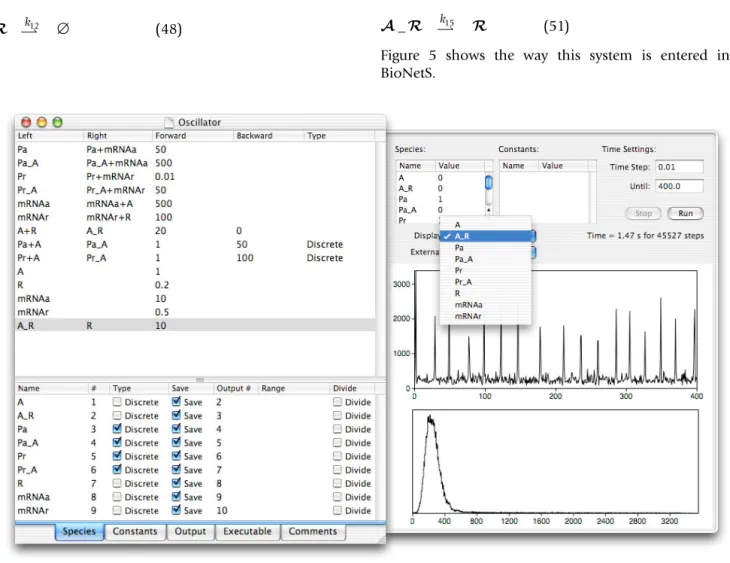
Figure 5 shows the way this system is entered into BioNetS.
An interesting feature of the system is that it is capable of producing sustained oscillations [37]. Figure 6A shows a times series for the repressor protein number when all the chemical species are treated as discrete random variables. The values of the rate constants used to generate this figure are listed in Fig. 5.
The chemical species Pa, Pr, Pr_A, and Pr_A are binary ran-dom variables: they can only take on the values 0 or 1.
Therefore, these species can not be approximated as con-tinuous random variables. All the other chemical species appear in sufficient quantities to justify the continuum approximation. Figure 6B shows a time series correspond-ing to Fig. 6A uscorrespond-ing the hybrid model. The hybrid model was run using the semi-implicit Euler method, and for these parameter values, runs 3 times faster than full model. Visually, the agreement between the two methods appears good. To test the accuracy of the Euler method, we
2 )r 2 ) k k r + 9 10 46 _ ( )
U
) k11 47 ∅ ( )X
4 k12 48 ∅ ( )X
mRNAaX
k13 ∅ (49) mRNArX
k14 ∅ (50) ) 4_X
k15 4 ( )51A screen shot of the BioNetS user interface for the chemical oscillator example Figure 5
A screen shot of the BioNetS user interface for the chemical oscillator example. The parameter values shown in the figure are the ones used to produce the results shown in Figs. 6, 7, 8. The area to the right of the reaction entry interface is a a testing panel provided by BioNetS to allow the user to enter rate constants and initial conditions, then examine the results of a run.
used BioNetS to construct 2-D histograms of R versus
mRN Ar. The results for the discrete and hybrid models are shown in Figs. 7B and 7B. To construct these histograms 10, 000 oscillations were used. Excellent agreement between the discrete and hybrid model is seen. This indi-cates that the hybrid model is accurately sampling the steady-state distribution. To verify that the hybrid model
faithfully captures the dynamics of the system, we com-puted the power spectra of both models. The results are shown in Figs. 8A and 8B. Again, excellent agreement is seen between the discrete and hybrid model.
Sample paths for the repressor protein number Figure 6
Sample paths for the repressor protein number. Panel A is the fully discrete case and Panel B is the hybrid model.
Time(s)
R(t)
Discrete
0
50
100
150
200
250
300
350
400
0
2000
4000
6000
8000
10000
Time(s)
R(t)
Hybrid
0
50
100
150
200
250
300
350
400
0
2000
4000
6000
8000
10000
A
B
An engineered promoter system
Using standard techniques in modern molecular biology, it is possible to design novel systems of promoter-gene pairs, such that virtually any desired regulatory network architecture may be instantiated; such networks are often called "synthetic gene networks." Recent
implementa-tions have included direct negative [22] and positive [23] feedback, a bistable switch [12], an oscillator [11], an intercellular communication system [38], and a bimodal self-activating system [39].
2-D histograms of repressor mRNA number versus repressor protein number Figure 7
2-D histograms of repressor mRNA number versus repressor protein number. Red indicates regions of large frequency (i.e., where the system spends a lot of time) and blue indicates regions of low frequency. Panel A is for the discrete system and Panel B is the hybrid model. Roughly 10, 000 oscillations were used to produce both plots.
Hybrid method
mRNA
RR
10
30
1
2
3
4
5
6
7
8
9
10
11
12
0
10
20
30
40
50
60
70
Discrete method
mRNA
RR
10
30
1
2
3
4
5
6
7
8
9
10
11
12
0
10
20
30
40
50
60
70
A
B
In this example, we use BioNetS to implement a model of a simple, open-loop network based around a novel engi-neered promoter, which has been designed and constructed by N. Guido and J. J. Collins at Boston Uni-versity. The promoter, called OROlac, combines the Olac,
OR1, and OR2 operator sites, so that it is repressed by the lac repressor protein (LacI) and activated by the lambda repressor protein (CI); see Fig. 9. Experiments have been conducted in which the promoter, along with other sites to produce the activator and repressor proteins, is inte-grated into a high copy number plasmid and inserted into a strain of Escherichia coli. The promoter's activity is
observed using a fluorescent reporter, Green Fluorescent Protein (GFP). A detailed modeling study with direct comparisons to experimental results has been carried out using a fully discrete stochastic approach, and will be reported elsewhere (McMillen et al., manuscript in prepa-ration). Our goal here is to provide a reasonably complex test case to evaluate the performance of BioNetS.
The processes to be captured by the model are: transcrip-tion and degradatranscrip-tion of mRNA strands; translatranscrip-tion of mRNA into protein; degradation of protein; formation of protein multimers (dimers in the case of CI, tetramers in Power spectra for the repressor protein number
Figure 8
Power spectra for the repressor protein number. Panel A is the discrete case and B is the hybrid model.
Hybrid
Frequency
Power
0
0.05
0.1
0.15
0.2
0.25
0.3
0.35
0.4
0.45
0.5
0
50
100
Discrete
Frequency
Power
0
0.05
0.1
0.15
0.2
0.25
0.3
0.35
0.4
0.45
0.5
0
50
100
A
B
the case of LacI); LacI binding to isopropyl-β-D-thioga-lactopyranoside (IPTG), a chemical inducer that reduces LacI's binding affinity for Olac; and protein-DNA binding at the OROlac promoter's operator sites. We define the fol-lowing chemical species: G, GFP; Mg, mRNA coding for GFP; X, CI monomer; X2, CI dimer; Mx, mRNA coding for CI; Dx, the arabinose-inducible pBAD promoter site producing CI; Y, LacI monomer; Y2, LacI dimer; Y4, LacI
tetramer; I0, IPTG (present in massive excess and thus taken to be constant); YI, LacI tetramer bound to IPTG; My, mRNA coding for LacI; and Dy, the PLtetO1 site
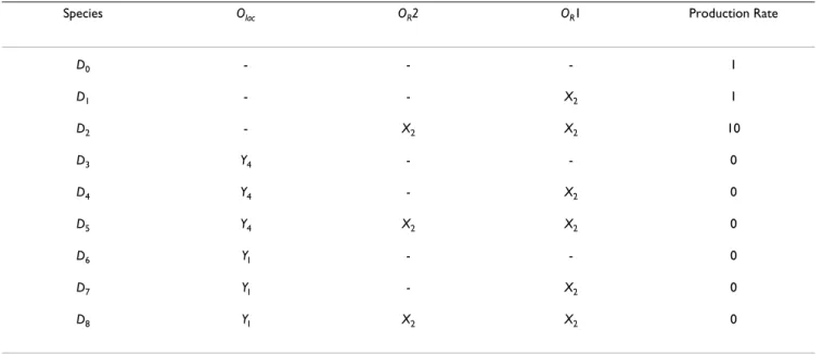
constitu-tively producing LacI. In addition to these, we define spe-cies D0 through D8, representing the various permutations
of proteins bound to the three operator sites in the OROlac
promoter (see Table for a list). There are twelve combina-torial possibilities, but we eliminate three of them on the basis that CI (X2) binding OR2 but notOR1 is unlikely, because of the low binding affinitity of CI for OR2 com-pared toOR1. Table also lists the effect on the basal rate of production when the promoter is in each state. This reflects the regulatory effect of the proteins; for example, CI bound to OR2 leads to a 10-fold increase in transcrip-tion rate, while LacI bound to Olac halts transcription com-pletely (note that we assume in the event of simultaneous
binding of activator and repressor, repression "wins" and transcription is halted).
The following irreversible reactions represent the proc-esses of transcription, translation, and degradation: Schematic of the OROlac engineered promoter
Figure 9
Schematic of the OROlac engineered promoter. The promoter fuses three operator sites, one of which (Olac) yields repression when the LacI tetramer is bound to it, while binding of the CI dimer to OR2 yields approximately ten-fold activation (the OR1 site assists activation by cooperatively enhancing CI binding to OR2 when CI is bound to OR1). In the experimental system, CI and LacI are produced in the cell by external promoters, not shown here. The Green Fluorescent Protein (GFP) product is then used to monitor the output of the promoter by flow cytometry.
O
lac
O
R1
O
R2
LacI
CI
GFP
D0 D0 M 52 βg g → + ( ) D1 D M1 53 βg g → + ( ) D2 D M 10 2 54 βg g → + ( ) Dy y Dy My β → + (55) Dx →βx Dx+Mx (56) Mg →βT Mg +G (57)As in previous reactions, the caligraphic letters represent individual molecules of each species. We scale all times and rates by the cell division time.
Experimental measurements generally provide equilib-rium rather than rate constants, and thus when writing reversible reactions we use the following notational con-vention: a reaction with equilibrium constant K has for-ward rate constant KR and backfor-ward rate constant R, where R is a scaling factor which sets the speed at which the reaction approaches equilibrium (we will consider three values of R: 1, 10, and 100). Using this notation, we represent protein-protein binding with the following set of reactions
Finally, protein-DNA binding is given by:
In all, the system consists of 21 species, participating in 34 reactions. The reactions are entered into BioNetS using the same method described in the previous examples. We use BioNetS' ability to represent individual species as either discrete or continuous to formulate three versions of the model: fully discrete, fully continuous, and a hybrid ver-sion in which the DNA species D0 through D8 are discrete while all other species are continuous. We vary the value of R, the scaling factor for reversible reactions, and keep all other parameters fixed at the following nondimension-alized values: βg = 0.1, βy = 1, βx = 0.5, βT = 10, γmrna = 3.5, γprot = 0.7, Ky = 0.01, Ky2 = 0.1, KyI = 2 × 10⁻⁶, K
x = 0.05, K1
= 0.3, K2 = 2K1,K3 = 0.008, K4 = 1.4 × l0-4K
3, I0 = 1 × 10⁶.
To evaluate the steady-state probability distributions pro-duced by the reaction system, simulations 250000 cell cycles in length were used to accumulate histograms (a built-in feature of BioNetS) of the number of molecules of GFP (species G), for each of the three versions of the model. As Fig. 10A shows, the resulting distributions are essentially identical, indicating that the continuum approximations used in the fully continuous and hybrid forms of the model were valid. Not all species in the
sys-My →βT My+Y (58) Mx →βT Mx +X (59) Mgγ ∅mrna→ (60) Myγ ∅mrna→ ( )61 Mxγ ∅mrna→ (62) /γ ∅prot→ ( )63 ;γ ∅prot→ (64) :γ ∅prot→ ( )65 ; ;+ Ky ; 2 ( )66
U
;2 ;2 ;4 2 67 + Ky ( )U
;4+I0 ; 68 K I yI ( )U
: :+ Kx : 2 ( )69U
,0+:2 1 ,1 70 K ( )U
,1+:2 2 ,2 71 K ( )U
,0+;4 3 ,3 72 K ( )U
,1+;4 3 ,4 73 K ( )U
,3+:2 1 ,4 74 K ( )U
,2+;4 3 ,5 75 K ( )U
,4+:2 2 ,5 76 K ( )U
,0+;I 4 ,6 77 K ( )U
,1+;I 4 ,7 78 K ( )U
,6+:2 1 ,7 79 K ( )U
,2+;I 4 ,8 80 K ( )U
,7+:2 2 ,8 81 K ( )U
tem are well approximated as continuous variables: Fig. 10B shows the continuous probability distribution for species D8, representing a promoter fully populated with two CI dimers and a LacI tetramer-IPTG complex. This sit-uation is very rare in our parameter regime, and the sys-tem spends essentially all of its time with D8 = 0. The fully continuous model, however, fluctuates into negative val-ues, indicating that the continuum approximation has broken down. This does not significantly affect the distri-bution for GFP because the other, more common DNA states dominate the system's behavior; note, however, that if we were considering genomic DNA rather than a high copy number plasmid, we would not be able to employ a fully continuous model. The hybrid model, by treating the DNA species as continuous, eliminates the fluctuations into negative values. In general, the appropriate approxi-mations will depend on both the system and the variables of interest: in the present example, if we were interested in the behavior of the operator sites themselves, we would not be able to use the fully continuous version of the model, but as a model solely of GFP expression the approximation suffices. Comparisons between types of models should be made to test the underlying assump-tions, and BioNetS facilitates this process.
We used simulations 200 cell cycles in length to test the speed at which the three model versions ran. In each case, 200 simulations were run using a consistent set of 200 dif-ferent random seeds; all runs were started with identical initial conditions. For the fully continuous and hybrid systems, the semi-implicit scheme was numerically stable and yielded consistent histograms for all time step sizes between dt = 0.001 and dt = 0.5, but the latter corresponds to just two time points per cell division cycle (recall that all times are scaled by the cell division time), and we chose instead to sample 20 points per cycle and set dt = 0.05. As shown in Table 2, the fully continuous method was always fastest, with the degree of improvement over the exact, fully discrete method depending strongly on the value of R, the scaling factor for the reversible reaction rates. For R = 1, the fully continuous method was only 1.4-fold faster than the fully discrete method, but as R is increased this speed advantage increases to over 4-fold at
R = 10, then to over 30-fold at R = 100. (Note that the
speed advantage of the fully continuous over the fully dis-crete method increases with the abundances of the chem-ical species. Shifting parameters to generate higher protein numbers can yield cases in which the continuum approx-imation is hundreds of times faster than the discrete approach; runs not shown here.) Use of a hybrid discrete/ continuous method did not, for this particular model sys-tem, offer any speed gain over the fully discrete approach; the increased time involved in computing the Jacobian for the semi-implicit method is more time-consuming than simply simulating the reactions directly. Optimizing
effi-ciency requires testing various potential approaches, and BioNetS makes this a simple process.
Conclusions
We have developed BioNetS to be a reliable tool for stud-ying the stochastic dynamics of large chemical networks. The software allows the user to specify which of the chem-ical species in the network should be treated as discrete random variables and which can be approximated as continuous random variables. The software is highly opti-mized for speed and should be be able to simulate net-works consisting of hundreds of chemical species. We have verified the accuracy of the numerical methods by considering several test systems (a dimerization reaction, a chemical oscillator, and an engineered promoter), each of which shows excellent agreement between the fully dis-crete version and the fully or partially continuous ver-sions. Our hope is that BioNetS, by providing a simple, user-friendly interface, will allow biological experimental-ists to formulate biochemical reaction models of their sys-tems quickly and easily, ideally increasing the number of systems in which direct comparisons are available between models and experimental results. Clearly, not every possible biological system can be captured in the current version of BioNetS, and its capabilities will con-tinue to grow in the future. We wish to encourage users, or potential users, to contact us regarding which additional features would be most helpful to them.
Availability and requirements
• Project name: BlOchemical NETwork Stochastic Simu-lator (BioNetS)
• Project home page: http://x.amath.unc.edu/BioNetS • Operating system:
* User interface: Macintosh OS X, version 10.2 or above. * Generated source code: Ability to compile portable C++ code. Makefiles included for OS X and Linux.
• Programming language: C++. • Other requirements: None. • License: BSD license.
• Restrictions on use by non-academics: None.
Authors' contributions
DA wrote the BioNetS code in its entirety, providing the user interface, the numerical optimizations and the code generator. TE provided the mathematical derivations, car-ried out the dimer and oscillator examples, wrote an
ini-tial draft of the paper, and worked with DA on the algorithms and numerical methods. DM revised and final-ized the paper, provided the engineered promoter exam-ple, and worked extensively with DA on testing and debugging of the software. All authors read, edited, and approved the final version of the paper.
A) Probability densities of GFP molecules, for three versions of the OROlac promoter model Figure 10
A) Probability densities of GFP molecules, for three versions of the OROlac promoter model. Densities were generated by accu-mulating statistics in runs 250000 cell cycles in duration. (Solid line) Fully discrete model. (Dashed line) Fully continuous model. (Dash-dotted line) Hybrid model: the DNA binding states are represented by discrete variables, while all other species are con-tinuous. All three methods produce virtually identical probability distributions. B) Probability density for species D8, for the continuous model. The hybrid and fully discrete methods produce identical distributions in which D8 spends 99.996% of the time at zero. This histogram shows that the continuous model artificially allows negative numbers (see inset time series).
D
8-6
-5
-4
-3
-2
-1
0
1
2
3
4
0
0.5
1
1.5
Discrete
Continuous
Hybrid
GFP
0
100
200
300
0
5
10
15
20
D
8vs time
20 40 60 80 100 -1 0 1A
B
Table 1: List of DNA-binding states in the OROlac engineered promoter example.
Species Olac OR2 OR1 Production Rate
D0 - - - 1 D1 - - X2 1 D2 - X2 X2 10 D3 Y4 - - 0 D4 Y4 - X2 0 D5 Y4 X2 X2 0 D6 YI - - 0 D7 YI - X2 0 D8 YI X2 X2 0
Column Olac represents the lac operator site, while columns OR1 and OR2 represent the two operator sites in the prm region of bacteriophage λ.
Entries in these columns indicate which regulatory proteins are bound to the operator sites in each state. The production rate column indicates
how quickly transcription from the promoter proceeds in each state: basal expression occurs in states D0 and D1; enhanced expression occurs in
state D2; and the remaining states display full repression (no expression).
Table 2: Execution times for three versions of the OROlac promoter model.
Fully continuous Fully discrete Hybrid
R Mean (s) Std (s) Mean (s) Std (s) Mean (s) Std (s)
1 0.26 [1] 0.01 0.36 [1.4] 0.01 0.69 [2.7] 0.01
10 0.27 [1] 0.01 1.15 [4.3] 0.01 6.91 [27] 0.12
100 0.27 [1] 0.01 9.11 [34] 0.28 69.43 [260] 1.13
The mean values represent the number of seconds of CPU time required to run a simulation of 200 cell cycles on an otherwise unloaded 700 MHz PowerPC G4 processor, averaged over a set of 200 different random seeds, identical for each version of the model. "Std" indicates the standard deviation of this same set of 200 runs. Three values of parameter R, a scaling factor giving the relative speed of the reversible reactions in the system, have been used. In each row, the values in square brackets are normalized by the shortest execution time. The fully continuous version runs substantially faster than the other methods, and its execution time does not depend on R. The fully continuous version produces identical
histograms to the fully discrete and hybrid methods for GFP (see Fig. 10A), but for the low-number species such as D8 it produces spurious negative
values (see Fig. 10B). If accuracy is required for the small-number states, the fully discrete method should be used; note that for this system, the hybrid approach is consistently slower than the fully discrete method.
Table 3
• Initialize all species and rate constants • Compute all reaction rates
• Loop:
* Set µ = sum of rates for the discrete reactions
* if (pt = µ∆t > ε), use Gillespie algorithm:
* R = a uniform random number in (0,1) * Set timeStep = -log(R)/µ
* Find which reaction occurred, update the species involved * else, use small ∆t approximation:
* R = a uniform random number in [0,1] * timeStep = continuousTimeStep
* if (R <pt = µ × timeStep), discrete transition has occurred:
• Determine which discrete transition occurred: • Find the first value of k for which
• If , the forward reaction occurred, otherwise the backward reaction occurred
* else, no discrete transition:
• No discrete reaction occurs, update is entirely due to continuous reactions (below) * end if (small ∆t method, determination if discrete transition occurred)
* end if (selection of Gillespie or small ∆t method for discrete reactions)
* Update the continuous species using the Langevin equation, with step size timeStep (where timeStep is either equal to continuousTimeStep or to the step size found by the Gillespie algorithm), using a semi-implicit numerical method
* Update any rates that have been changed by the continuous reactions and the single discrete reaction * Break when user-defined total simulation time is reached
• end loop [Fi Bi] R i k + ≥ =
∑
1 µ [Fi Bi] Fk R i k + + ≥ =−∑
11 µPublish with BioMed Central and every scientist can read your work free of charge "BioMed Central will be the most significant development for disseminating the results of biomedical researc h in our lifetime."
Sir Paul Nurse, Cancer Research UK
Your research papers will be:
available free of charge to the entire biomedical community peer reviewed and published immediately upon acceptance cited in PubMed and archived on PubMed Central yours — you keep the copyright
Submit your manuscript here:
http://www.biomedcentral.com/info/publishing_adv.asp
BioMedcentral
Acknowledgements
This work was supported by DARPA grant F30602-01-2-0579. D. Adal-steinsson acknowledges support by the Alfred P. Sloan Foundation.
References
1. Glass L, Kauffman S: The logical analysis of continuous, nonlin-ear biochemical control networks. J Theor Biol 1973, 39:103-129. 2. Kauffman S: The large-scale structure and dynamics of gene control circuits: An ensemble approach. J Theor Biol 1974, 44:167-190.
3. Savageau M: Comparison of classical and autogenous systems of regulation in inducible operons. Nature 1974, 252:546-549. 4. Glass L: Classification of biological networks by their
qualita-tive dynamics. J Theor Biol 1975, 54:85-107.
5. Tyson J, Othmer H: The dynamics of feedback control circuits in biochemical pathways. Progr Theor Biol 1978, 5:1-60.
6. Ackers G, Johnson A, Shea M: Quantitative model for gene reg-ulation by λ phage repressor. Proc Natl Acad Sci USA 1982, 79:1129-1133.
7. Shea M, Ackers G: The OR control system of bacteriophage
lambda: A physical-chemical model for gene regulation. J Mol Biol 1985, 181:211-230.
8. Reinitz J, Vaisnys J: Theoretical and experimental analysis of the phage lambda genetic switch implies missing levels of co-operativity. J Theor Biol 1990, 145:295-318.
9. Keller A: Model genetic circuits encoding autoregulatory transcription factors. J Theor Biol 1995, 172:169-185.
10. Mestl T, Lemay C, Glass L: Chaos in high-dimensional neural and gene networks. Physica D 1996, 98:33-52.
11. Elowitz M, Leibler S: A synthetic oscillatory network of tran-scriptonal regulators. Nature 2000, 403:335-338.
12. Gardner T, Cantor C, Collins J: Construction of a genetic toggle switch in Escherichia coli. Nature 2000, 403:339-342.
13. Endy D, You L, Yin J, Molineux I: Computation, prediction, and experimental tests of fitness for bacteriophage T7 mutants with permuted genomes. Proc Natl Acad Sci USA 2000, 97:5375-5380.
14. Hasty J, Isaacs F, Dolnik M, McMillen D, Collins J: Designer gene networks: Towards fundamental cellular control. Chaos 2001, 11:207-220.
15. Santillán M, Mackey M: Dynamic regulation of the tryptophan operon: A modeling study and comparison with experimen-tal data. Proc Natl Acad Sci USA 2001, 98:1364-1369.
16. McMillen D, Kopell N, Hasty J, Collins J: Synchronizing genetic relaxation oscillators by intercell signaling. Proc Natl Acad Sci USA 2002, 99:679-684.
17. Spudich J, Koshland DEJ: Non-genetic individuality: Chance in the single cell. Nature 1976, 262:467-471.
18. Ross I, Browne C, Hume D: Transcription of individual genes in eukaryotic cells occurs randomly and infrequently. Immunol Cell Biol 1994, 72:177-185.
19. Hume D: Probability in transcriptional regulation and its implications for leukocyte differentiation and inducible gene expression. Blood 2000, 96:2323-2328.
20. Arkin A, Ross J, McAdams H: Stochastic kinetic analysis of devel-opmental pathway bifurcation in phage λ -infected Escherichia coli cells. Genetics 1998, 149:1633-1648.
21. Barkai N, Leibler S: Biological rhythms: Circadian clocks lim-ited by noise. Nature 2000, 403:267.
22. Becskei A, Serrano L: Engineering stability in gene networks by autoregulation. Nature 2000, 405:590-593.
23. Becskei A, Séraphin B, Serrano L: Positive feedback in eukaryotic gene networks: cell differentiation by graded to binary response conversion. EMBO J 2001, 20:2528-2535.
24. Bialek W: Stability and noise in biochemical switches. In Advances in Neural Information Processing Systems Volume 13. Cam-bridge: The MIT Press; 2001:103-109.
25. Elowitz M, Levine A, Siggia E, Swain P: Stochastic gene expression in a single cell. Science 2002, 297:1183-1186.
26. Hasty J, Pradines J, Dolnik M, Collins J: Noise-based switches and amplifiers for gene expression. Proc Natl Acad Sci USA 2000, 97:2075-2080.
27. Ko M: A stochastic model for gene induction. J Theor Biol 1991, 153:181-194.
28. Kepler T, Elston T: Stochasticity in transcriptional regulation: origins, consequences, and mathematical representations. Biophys J 2001, 81:3116-3136.
29. McAdams H, Arkin A: Stochastic mechanisms in gene expression. Proc Natl Acad Sci USA 1997, 94:814-819.
30. Ozbudak E, Thattai M, Kurtser I, Grossman A, van Oudenaarden A: Regulation of noise in the expression of a single gene. Nature Genet 2002, 31:69-73.
31. Thattai M, van Oudenaarden A: Intrinsic noise in gene regulatory networks. Proc Natl Acad Sci USA 2001, 98:8614-8619.
32. Gillespie D: Exact stochastic simulation of coupled chemical reactions. J Phys Chem 1977, 81:2340-2361.
33. Gibson M, Bruck J: Efficient exact stochastic simulation of chemical systems with many species and many channels. J Phys Chem 2000, 104:1876-1889.
34. Gillespie D: Approximate accelerated stochastic simulation of chemically reacting systems. J Phys Chem 2001, 115:1716-1733. 35. Gardiner C: Handbook of stochastic methods: For physics, chemistry and
the natural sciences Berlin: Springer Verlag; 1996.
36. Kloeden P, Platen E: Numerical solution of stochastic differential equations Berlin: Springer Verlag; 1992.
37. Vilar J, Kueh H, Barkai N, Leibler S: Mechanisms of noise-resist-ance in genetic oscillators. Proc Natl Acad Sci USA 2002, 99:5988-5992.
38. Weiss R, Knight T: Engineered communications for microbial robotics. In DNA6: Sixth International Meeting on DNA Based Comput-ers: June 13–17 2000; Leiden, Netherlands Edited by: Condon A, Rozen-berg G. Berlin: Springer Verlag; 2001.
39. Isaacs F, Hasty J, Cantor C, Collins J: Prediction and measure-ment of an autoregulatory genetic module. Proc Natl Acad Sci USA 2003, 100:7714-7719.