Abstract— The functions of 3R Planar Robot Arm are described in this journal. It includes three main parts: first is calculation of inverse kinematics of robot arm, second is sending joint angle values to ARDUINO by serial communication and another is ARDUINO drive the arm. In which, three motors are used to move the arm. When the desired input (x, y and ϕ) are entered, inverse kinematic in the MATLAB program in PC is calculated joint angle values and then send it to the ARDUINO. This research used the MATLAB software to calculate the inverse kinematic of robot arm and also uses it as a graphical user interface (GUI) for controlling the movement of this robot. If the ARDUINO get the joint angle values, the motor drives the arm.
Index Terms— Interface, MATLAB, Forward Kinematics, Inverse Kinematics, Trajectory.
1) INTRODUCTION
Robotics education has been based on mobile robotics and manipulator-based robotics. Manipulator-based robotics education requires a large start up investment. This thesis is concerned with the fundamentals of robotics, including kinematics, computer interfacing, and control concepts as applied to industrial robot manipulators. The mathematical modelling of spatial linkages is quite involved. It is useful to start with planar robots because the kinematics of planar mechanisms is generally much simpler to analyze. A link parameter link length and link twist defines the relative location of the two axes in space. A link parameter is link length and link twist. The link offset is the distance between two consecutive links along the axis of the joint. The joint angle is the rotation of one link with respect to the next about the joint axis. These four parameters together are called Denavit-Hartenberg (D-H) parameters. The end effectors position can be controlled using either the joint angle or the link offset.
The forward kinematics problem is concerned with the relationship between the individual joints of the robot manipulator and the position and orientation of the tool or end-effector. The inverse problem of finding the joint variables in terms of the end effector position and orientation is the problem of inverse kinematics and it is in general more difficult than the forward kinematics problem. Deriving both forward and inverse kinematics is an important step in robot modelling based on Denavit -Hartenberg (D-H) representation [1].
One of the most common requirements in robotics is to move the end-effector smoothly from one pose to another
Manuscript received Oct, 2017.
Moe Thu Zar, Mechatronic Engineering Department, Mandalay Technological University, Mandalay, Myanmar, +959786060301.
Wai Phyo Ei, Mechatronic Engineering Department, Mandalay
Technological University, Mandalay, Myanmar.
pose. The control objective is to make the 3R robot manipulator traces desired trajectory. There are two approaches to generating such trajectories known respectively as joint-space and Cartesian motion. In this research, Cartesian space or operational space trajectory is used. PID tuning software method (eg. MATLAB) are used in this research.
2) SYSTEM BLOCK DIAGRAM OF PLANAR ROBOT ARM The complete system block diagram shown in Figure 1 consists of many parts like, personal computer with serial communication adapter, ARDUINO, servo, potentiometer and robot arm. Firstly, when the program is run, inverse kinematics in MATLAB is calculating the joint angle value and then sending data to ARDUINO that drives the robot arm. The main function of the ARDUINO is sending joint angle values to the servo motors, feeding the joint angle values from encoders of the servo motors and send back to the ARDUINO. + Sensor (potentiometer) Robot Arm _ Position Reference Position Actuator (servo) Computer MATLAB ARDUINO PID
Figure.1. Overall Block Diagram of the System.
3) ROBOTIC ANALYSIS
The analysis of a robot consists of determining D-H parameters, calculating robot kinematics and dynamics, and controlling the robot via a control scheme. The control scheme may be PID, Fuzzy, NN or Visual Control.
i. Determining D-H Parameters
D-H parameters table is a notation developed by Denavit and Hartenberg, is intended for the allocation of orthogonal coordinates for a pair of adjacent links in an open kinematic system. It is used in robotics, where a robot can be modelled as a number of related solids (segments) where the D-H parameters are used to define the relationship between the two adjacent segments. The first step in determining the D-H parameters is locating links and determines the type of movement (rotation or translation) for each link.
Point to Point Trajectory Control of 3R Planar
Robot Arm
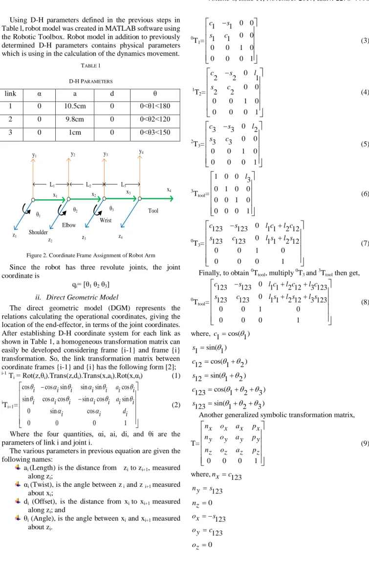
Using D-H parameters defined in the previous steps in Table l, robot model was created in MATLAB software using the Robotic Toolbox. Robot model in addition to previously determined D-H parameters contains physical parameters which is using in the calculation of the dynamics movement.
TABLE 1 D-HPARAMETERS link α a d θ 1 0 10.5cm 0 0<θ1<180 2 0 9.8cm 0 0<θ2<120 3 0 1cm 0 0<θ3<150 Shoulder Elbow Wrist Tool x1 x2 x3 x4 y1 y2 y3 y4 z1 z2 z3 z4 L1 L2 L3 θ1 θ2 θ3
Figure 2. Coordinate Frame Assignment of Robot Arm
Since the robot has three revolute joints, the joint coordinate is
qi= [θ1 θ2 θ3]
ii. Direct Geometric Model
The direct geometric model (DGM) represents the relations calculating the operational coordinates, giving the location of the end-effector, in terms of the joint coordinates. After establishing D-H coordinate system for each link as shown in Table 1, a homogeneous transformation matrix can easily be developed considering frame {i-1} and frame {i} transformation. So, the link transformation matrix between coordinate frames {i-1} and {i} has the following form [2];
i-1
Ti = Rot(z,θi).Trans(z,di).Trans(x,ai).Rot(x,αi) (1)
i
Ti+1=
cos cos sin sin sin cos
sin cos cos sin cos sin
0 sin cos 0 0 0 1 a i i i i i i i a i i i i i i i d i i i
(2)Where the four quantities, αi, ai, di, and θi are the parameters of link i and joint i.
The various parameters in previous equation are given the following names:
ai (Length) is the distance from zi to zi+1, measured
along zi;
αi (Twist), is the angle between z i and z i+1 measured
about xi;
di (Offset), is the distance from xi to xi+1 measured
along zi; and
θi (Angle), is the angle between xi and xi+1 measured
about zi. 0 T1= 0 0 1 1 0 0 1 1 0 0 1 0 0 0 0 1 c s s c
(3) 1 T2= 0 2 2 1 0 0 2 2 0 0 1 0 0 0 0 1 c s l s c
(4) 2 T3= 0 3 3 2 0 0 3 3 0 0 1 0 0 0 0 1 c s l s c
(5) 3 Ttool= 1 0 0 3 0 1 0 0 0 0 1 0 0 0 0 1 l
(6) 0 T3= 0 123 123 1 1 2 12 0 123 123 1 1 2 12 0 0 1 0 0 0 0 1 c s l c l c s c l s l s
(7)Finally, to obtain 0Ttool, multiply 0T3 and 3Ttool then get,
0 Ttool= 0 123 123 1 1 2 12 3 123 0 123 123 1 1 2 12 3 123 0 0 1 0 0 0 0 1 c s l c l c l c s c l s l s l s
(8) where, c1cos(1) sin( ) 1 1 s cos( ) 12 1 2 c sin( ) 12 1 2 s cos( ) 123 1 2 3 c sin( ) 123 1 2 3 s Another generalized symbolic transformation matrix,
T= 0 0 0 1 nx ox ax px ny oy ay py nz oz az pz
(9) where,nxc123 123 ny s 0 nz 123 ox s 123 oy c 0 oz 0 ax 0 a y 1 az 1 1 2 12 3 123 px l c l c l c 1 1 2 12 3 123 py l s l s l s 0 pz
iii. Inverse Geometric Model
Manipulator solution strategies into two broad classes: closed-form solutions and numerical solutions. Because of their iterative nature, numerical solutions generally are much slower than the corresponding closed-form solution. For most uses, are not interested in the numerical approach to solution of kinematics [3]. Within the class of closed-form solutions, distinguish two methods of obtaining the solution: algebraic and geometric. Inverse kinematic need to find the joint angle , and ,corresponding end effector’s position and orientation. For a planar motion, the position and orientation of the end effector can be specified by the origin of the frame 4, i.e (px, py) and the orientation of the frame attached to the end effector with respect to X axis, i.e. angle ϕ. X Y θ1 θ2 θ3 Φ=θ1+θ2+θ3 a1 a2 a3
Figure 3. 3-DOF (3R) Planar Robot Arm
For the simulation of the inverse kinematics for 3R planar robot arm, these equations can be simplified as follows:
c c c 1 1 2 12 3 123 px a a a (10) s s s 1 1 2 12 3 123 py a a a (11) 1 2 3 (12) The coordinate of wrist is
w
x andw
y:cos( ) c c 3 1 1 2 12 wx pxa a a (13) sin( ) s s 3 1 1 2 12 wy pya a a (14) Squaring the two sides of equation (13) and (14),
2 2 2 2 2 cos( ) 1 2 1 2 2 wx wy a a a a 2 2 2 2 1 2 cos( 2) 2 1 2 wx wy a a a a (15) 2 1 2 2 s c (16) tan 2( , ) 2 a s2 2c (17) By expanding cos(12)and sin(12)of equation (13) and (14), and rearranging them as:
( 1 2 2c ) c1 2 1 2s s wx a a a (18) ( 1 2 2c ) s1 2 1 2c s wy a a a (19) ( 1 2cos( 2)) 2 2 1 2 2 a a wy a s wx s wx wy (20) ( 1 2cos( 2)) 2 2 1 2 2 a a wx a s wy c wx wy (21) tan 2( , ) 1 a s c1 1 (22) 3 1 2 (23) 4) ROBOT HARDWARE AND SOFTWARE
To achieve a control of a robot arm by using personal computer, it must make the connection between the robot and PC. This connection is called interface connection and it is done by using a ARDUINO. ARDUINO is designed to interface to and interact with electrical/electronic devices, sensors and actuators, and high-tech gadgets to automate systems. The complete control process can be divided into two categories, hardware and software.
A. Hardware Environment
The hardware environment for this thesis consists of a ARDUINO, a PC, and a data link between the PC and robot arm. The ARDUINO is a device that interfaces to sensors and robot actuators and performs embedded computing. The PC is used to control the robot by GUI; it is used to write the user defined embedded program which is to be run on the ARDUINO. In this thesis, use a serial communication link(wire) between the ARDUINO and PC.
Figure.4. Hardware Environment i. Arduino
The Arduino Mega 2560 is a microcontroller board based on the ATmega2560 (datasheet). It has 54 digital input/output pins (of which 14 can be used as PWM outputs), 16 analog inputs, 4 UARTs (hardware serial ports), a 16 MHz crystal oscillator, a USB connection, a power jack, an ICSP header,
and a reset button. It contains everything needed to support the microcontroller; simply connect it to a computer with a USB cable or power it with a AC-to-DC adapter or battery to get started. The Mega is compatible with most shields designed for the Arduino Duemilanove or Diecimila.
ii. Personal Computer
As previously mentioned, the PC is used to write Basic programs that the ARDUINO executes and to display sensory data processed by the ARDUINO and control the robot using MATLAB GUI. Any PC that supports MATLAB can be used.
iii. Servo Motor
Servo control in general can be broken into two fundamental classes of problems. The first class deals with command tracking. It addresses the question of how well does the actual motion follow what is being commanded. The typical commands in rotary motion control are position, velocity, acceleration and torque. The second general class of servo control addresses the disturbance rejection characteristics of the system. Disturbances can be anything from torque disturbances on the motor shaft to incorrect motor parameter estimations used in the feedforward control.
Figure.5. Servo Motor (MG995_Tower-Pro) B. Software Environment
Software environment can be divided into two parts: the ARDUINO program and MATLAB Program. In ARDUINO program, write a code to make the interfacing between PC and arm. The MATLAB program consists of the Serial Communication code and the graphical user interface (GUI).
5) OPERATION OF THE CONTROL SYSTEM MATLAB and ARDUINO program is applied in this research.
When the inverse kinematic of the robot arm is calculated, MATLAB sends joint angle value as serial data to the robot. By entering each corresponding input, the operator can control simultaneously the robot movement. While performing these actions, the operator can check whether the command is correct or not with the help of LCD display.
All the motors are driven by the joint angle values received from the MATLAB in PC. ARDUINO is also used as the main microcontroller to interface with other devices by receiving the data. The robot is moved to the desired position with the help of three servo motors and another one servo motor is used to move the ball-pen up and down to write some numbers.
6) ALGORITHM OF TRAJECTORY CONTROL SYSTEM Straight-line motions are most common in the industrial applications; however, movement on a line is mostly
obtained by specifying the discrete time joint- displacements at a constant time rate. The velocity and acceleration of the points can be calculated from the numerical approximation of the time derivatives. Several methods were used to compress the describing data of the trajectories as cubic, quintic and LSPB trajectory.
Cubic Trajectory: Cubic polynomial or third order polynomial approximation describes the path parametrically as a function of time with the position and velocity constraints at initial time t = zero and final time tf. It gives continuous positions and velocities at the start and finish points times but discontinuities in the acceleration. The derivative of acceleration is called the jerk. Higher order polynomials are required to guarantee the smoothness of the joint accelerations.
Quintic Trajectory: A discontinuity in acceleration leads to an impulsive jerk, which may excite vibration modes in the manipulator and reduce tracking accuracy. For this reason, one may wish to specify constraints on the acceleration as well as on the position and velocity. In this case, we have six constraints (one each for initial and final configurations, initial and final velocities, and initial and final accelerations). Therefore, a fifth order polynomial is required.
for distance: 0 2 3 4 5 ( ) 1 2 3 4 5 q q t a a ta t a t a t a t for velocity: . 2 3 4 ( ) 1 2 2 3 3 4 4 5 5 v q t a a t a t a t a t for acceleration: .. 2 3 ( ) 2 2 6 3 12 4 20 5 q t a a t a t a t
Figure 6. Quintic Polynomial Trajectory with Zero-Velocity Boundary Conditions [t0=0, tf=50 second, q0=0, qf=1, v=0 and α=0]
Figure 7. Quintic Polynomial Trajectory with Velocity Boundary Conditions [t0=0, tf=50 second, q0=0, qf=1, v0=0.5, vf=0 and α=0]
LSPB trajectory: Another way to generate suitable joint space trajectories is by so-called Linear Segments with Parabolic Blends or (LSPB) for short. This type of trajectory is appropriate when a constant velocity is desired along a portion of the path. The LSPB trajectory is such that the velocity is initially “ramped up” to its desired value and then “ramped down” when it approaches the goal position. To achieve this, we specify the desired trajectory in three parts. The first part from time t0 to time tb is a quadratic polynomial. This results in a linear “ramp” velocity. At time tb, called the blend time, the trajectory switches to a linear function. This corresponds to a constant velocity. Finally, at time tf − t b the trajectory switches once again, this time to a quadratic polynomial so that the velocity is linear [4][5].
2 0 2 0 ( ) 2 2 2 2 2 a q t q q Vt f f q t Vt atf a qf at tf t
Figure 8. LSPB with Zero-Velocity Boundary Conditions [t0=0, tf=50 second, q0=0, qf=1, v=0 and α=0]
Figure 9. LSPB with Velocity Boundary Conditions [t0=0, tf=50 second, q0=0, qf=1, v0[maximum]=0.035, v0[minimum]=0.025, vf=0, and α=0]
At home position all angles are zero, put θ1 = 0, θ2 = 0, θ3 = 0.
So the transformation matrix reduced to:
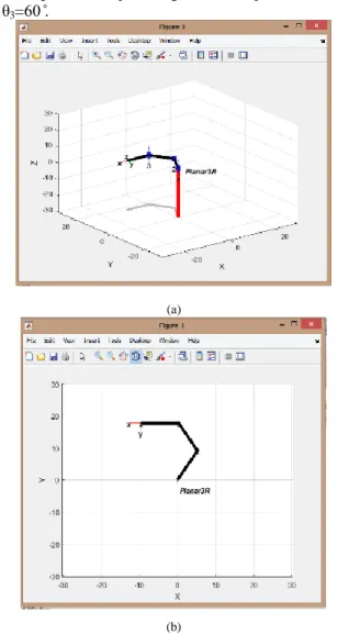
Figure 10. Visualization of robot in all zero joint angles in 3D and 2D At this position all joint angles are 60 ̊, put θ1=60 ̊, θ2=60 ̊
and θ3=60 ̊.
(a)
(b)
Figure.11. Visualization of robot in all 60 ̊ joint angles [ (a) 3D and (b) 2D view]
7) RESULTS AND DISCUSSIONS
The user enters the input position into the left three edit boxes for moving the base motor, first joint motor and second joint motor. MATLAB program is calculated the joint angle values by using inverse kinematic equation of the robot arm and then send to the microcontroller. Microcontroller receives these signals and then the motors rotate according to the instructed direction. MATLAB simulation result of the robot arm is shown in Figure 12.
0 t t
b
t
b
t t
f
t
b
Figure.12. Simulation Result of Serial Interfacing for Robot Arm in MATLAB Form
From home position, (x=30.3cm, y=0 cm and ϕ=0) to goal points is shown in Figure 13, Figure 14 and Figure 15.
Figure.13. Testing Photo of Robot Arm Control System for Home Position (x=30.3cm, y=0 cm and ϕ=0)
Figure.14. Testing Photo of Robot Arm Control System from Home Position to Goal Position (x=12 cm, y=10 cm and ϕ=90 ̊)
Figure.15. Testing Photo of Robot Arm Control System from Home Position to Goal Positions (x=16 cm, y=10 cm and x =10 cm, y=10 cm with φ=45 ̊)
The trajectory traced by the end effector with respect to original points. It is seen that at every point some error is occurring. This may be due to inaccuracies in the model setting including the motor clearance as well as due to the integer values of joint angles given to the ARDUINO program. The precision of robot arm is 2 cm.
Since MATLAB is slow in the execution time, recommend using a high-level computer programming language to perform the software part.
CONCLUSIONS
This journal represents a writing robot using PC based point to point trajectory control and it is designed for only as a sample. The Graphical User Interface (GUI) of the software package was developed for testing motional characteristics of the robot arm. A physical interface between the robot arm and the GUI was designed and built. A comparison between kinematics solutions of the virtual arm and the robot's arm physical motional behaviours have been accomplished. The results are displayed in a graphical format and the motion of all joints and end effector can be observed. Many future developments can be carried on this robot arm like other types for robots, these developments include path-planning, dynamics modelling, force control and computer vision.
ACKNOWLEDGEMENT
The author is deeply gratitude to Dr. Sint Soe, Rector of Mandalay Technological University (MTU) for his kind permission to submit this research. The author would like to thank to her supervisor, Daw Wai Phyo Ei, Lecturer of Mechatronic Engineering Department, Mandalay Technological University, for her valuable supervision guidance and comments for preparation of the research. After that, the author would like to thank Dr. Sint Soe, Associate Professor and thanks to all her teachers from Mechatronic Department, Mandalay Technological University.
REFERENCES
[1] MAHMOUD A. ABUALSEBAH, “Trajectory Tracking Control of
3-Dof Robot Manipulator Using Tsk Fuzzy Controller”, AUGUST
2013.
[2] J J. DENAVIT, R.S. HARTENBERG, “A Kinematics Notion
For Lower-Pair Mechanisms Based On Atrices”, ASME JOURNAL
OF APPLIED MECHANICS, VOL. 22, PP. 215–221, 1955. [3] PAUL R.C.P., “Robot Manipulators: Mathematics, Programming
[4] MOHAMMED REYAD ABUQASSEM, “Simulation and Interfacing
of 5 Dof Educational Robot Arm”, DEGREE OF MASTER OF
SCIENCE IN ELECTRICAL ENGINEERING, JUNE 2010 [5] PETER CORKE, “Robotics, Vision and Control”.

![Figure 6. Quintic Polynomial Trajectory with Zero-Velocity Boundary Conditions [t 0 =0, t f =50 second, q 0 =0, q f =1, v=0 and α=0]](https://thumb-us.123doks.com/thumbv2/123dok_us/8211726.2177196/4.893.464.782.487.870/figure-quintic-polynomial-trajectory-velocity-boundary-conditions-second.webp)