R E S E A R C H
Open Access
Simulation of a highly elastic structure
interacting with a two-phase flow
Erik Svenning, Andreas Mark
*and Fredrik Edelvik
*Correspondence:
[email protected] Fraunhofer-Chalmers Centre, Chalmers Science Park, Gothenburg, 412 88, Sweden
Abstract
Purpose:The aim of this paper is to present and validate a modeling framework that can be used for simulation of industrial applications involving fluid structure
interaction with large deformations.
Background:Fluid structure interaction phenomena involving elastic structures frequently occur in industrial applications such as rubber bushings filled with oil, the filling of liquid in a paperboard package or a fiber suspension flowing through a paper machine. Simulations of such phenomena are challenging due to the strong coupling between the fluid and the elastic structure. In the literature, this coupling is often achieved with an arbitrary Lagrangian Eulerian framework or with smooth particle hydrodynamics methods. In the present work, an immersed boundary method is used to couple a finite volume based Navier-Stokes solver with a finite element based structural mechanics solver for large deformations.
Results:The benchmark of an elastic rubber beam in a rolling tank partially filled with oil is simulated. The simulations are compared to experimental data as well as numerical simulations published in the literature. 2D simulations performed in the present work agree well with previously published data. Our 3D simulations capture effects neglected in the 2D case, showing excellent agreement with previously published experiments.
Conclusions:The good agreement with experimental data shows that the developed framework is suitable for simulation of industrial applications involving fluid structure interaction. If the structure is made of a highly elastic material, e.g. rubber, the simulation framework must be able to handle the large deformations that may occur. Immersed boundary methods are well suited for such applications, since they can efficiently handle moving objects without the need of a body-fitted mesh. Combining them with a structural mechanics solver for large deformations allows complex fluid structure interaction problems to be studied.
Keywords: fluid structure interaction; immersed boundary methods; sloshing tank; FSI benchmark
Introduction
Numerical simulations of highly elastic structures deforming in a free surface flow are challenging since the fluid-structure coupling is strong. The geometrically nonlinear re-sponse of the structure and the need to accurately resolve the free surface further increases the complexity of the simulations. The coupling between the fluid and the structure can be handled in different ways. A popular approach is the Arbitrary Lagrangian Eulerian (ALE) method [], where the grid is deformed when the structure moves. Simulations
with Smooth Particle Hydrodynamics (SPH) [, ] and Particle Finite Element Methods (PFEM) [] are also reported in the literature. Immersed Boundary Methods (IBM) al-low the flow around deforming objects in the flow to be resolved without the need of a body-fitted mesh. IBMs are therefore well suited for Fluid Structure Interaction (FSI) ap-plications with large structural displacements. The original IBM developed by Peskin [] was explicitly formulated and only first-order accurate in space. Majumdar et al. [] devel-oped a more stable method, which is implicitly formulated and second-order accurate in space. However, this method suffers from problems with mass conservation and pressure oscillations. To resolve these issues, Mark et al. [, ] developed a second-order accurate hybrid IBM. The IBM developed by Mark et al. has been validated for simulation of fiber suspension flows with elastic fibers in [].
FSI simulations can be performed in a monolithic or a partitioned way. Using a mono-lithic approach implies that all equations are solved simultaneously in the same matrix. In the partitioned approach, the different equations are solved separately and coupling algorithms are employed. Using the partitioned approach without coupling iterations be-tween the fluid and the structure solutions is attractive in terms of computational effi-ciency. However, this approach often results in instabilities due to the added mass effect if the simulation time is long enough []. Gauss-Seidel iterations as well as quasi-Newton [] techniques have been proposed to deal with these problems.
The aim of this paper is to present and validate a modeling framework that can be used for simulation of FSI in industrial applications. To achieve this, the partitioned approach with Gauss-Seidel iterations is used. The fluid-structure coupling is handled with the IBM developed by Mark et al. [] and the structure is modeled as a St. Venant-Kirchhoff mate-rial, thus taking large deformations into account.
Theory
In the present work, a finite volume discretization on a Cartesian octree grid is used to solve the Navier-Stokes equations. A finite element discretization in total Lagrangian for-mulation is used to predict the motion of the structure. The fluid and structure models together with the FSI coupling are described in the following.
Fluid model
The motion of an incompressible fluid is modeled by the Navier-Stokes equations:
∇ · u= , ()
ρf
∂u
∂t +ρfu· ∇u= –∇p+μ∇
u, ()
or the Volume Of Fluid (VOF) method. In both methods an additional scalar transport equation is solved,
∂
∂t +u· ∇= , ()
whereis the transported scalar. In the level set method a scalar field is convected and the interface between the two fluids is defined as a specified iso-surface. Hence, at each time step the phase of each computational cell is determined by a simple scalar comparison test. In this way the interface is kept sharp but the mass is not conserved. In the VOF method, that is used in the present work, a volume fractionαis defined and transported by the additional transport equation (=α). The density of the fluid is then defined as
ρf =ρoα+ ( –α)ρa, ()
whereρois the oil density andρais the air density. In this way the mass is conserved but the interface may be diffusive. Therefore, it is important to use a shock capturing con-vective scheme. Hence, in this work the shock capturing scheme CICSAM developed by Ubbink [] is employed. To further reduce the diffusion of the interface and improve the computational speed adaptive grid refinements along the interface are employed. The Backward Euler scheme is used for the temporal discretization.
Structure model
A deformable solid object is modeled as an elastic continuum. In the present work, large deformations as well as inertia effects are taken into account. The balance of linear mo-mentum in a continuum point is given by []
∇ ·σ+ρb–ρa=, ()
where σ is the Cauchy stress, bis the volume force (e.g. gravity),ais the acceleration,
ρ denotes density and∇·is the divergence operator. The balance equation for angular momentum can be used to derive the symmetry of the Cauchy stress, see e.g. []. As a consequence, only the balance of linear momentum needs to be solved in the structure simulation. Letδvdenote an arbitrary virtual velocity []. The spatial virtual work equa-tion, i.e. the weak form of (), can then be written as
δW=
v
(∇ ·σ+ρb–ρv˙)·δv dV = , ()
whereVdenotes volume of the body in the current configuration. The spatial virtual work equation above can be transformed into the material virtual work equation, so that the second Piola-Kirchhoff stressSappears as stress measure instead of the Cauchy stressσ. The relation between the Cauchy stress and the second Piola-Kirchhoff stress is given by
whereFis the deformation gradient andJ=detF. Large deformations can then be taken into account by using hyperelastic material models, that provide the relation between the second Piola-Kirchhoff stress and its work conjugate strain measure, the Green strainE.
The Green strainEis computed from the deformation gradientFaccording to
E=
FT·F–I. ()
In the present work, St. Venant-Kirchhoff elasticity is assumed, with a strain energy po-tential given by []
=
λ(trE)
+μE:E, ()
whereλandμare material parameters. The second Piola-Kirchhoff stress corresponding to equation () is
S=λ(trE)I+ μE. ()
The elasticity tensor corresponding to equation () is
Cijkl=
∂S
∂E=λδijδkl+μ(δikδjl+δilδjk), ()
whereδijdenotes the Kroenecker delta.
It is interesting to note that equation () is similar to the corresponding equation for lin-ear elasticity, but in equation () the Green strain applin-ears instead of the small strain ten-sor and the second Piola-Kirchhoff stress appears instead of the Cauchy stress. It should be mentioned that there are other material models for rubber, e.g. the Mooney-Rivlin model []. Such models offer higher accuracy at large strains, but require more input data for calibration. In the cases considered in the present work, the strains remain relatively small and the St. Venant-Kirchhoff model is therefore sufficient.
The Finite Element Method (FEM) is used to discretize the equations governing the motion of the solid. Isoparametric basis functions are used and the integrals are evalu-ated with Gaussian quadrature. Full integration is used in the simulations in the present work. The nonlinear system of equations is solved with Newton’s method, so that asymp-totic second order convergence in the iterations is achieved. Using Newton’s method re-quires computation of the consistent tangent stiffness matrix. This topic is well described in many books on FEM for structural mechanics, see e.g. [, ]. A pure displacement for-mulation is employed (in contrast to mixed forfor-mulations sometimes used, see e.g. []). Therefore, incompressible solid materials are modeled as nearly incompressible by setting Poisson’s ratio to a value close to, but not equal to, .. Hexahedral elements with -nodes are used in the simulations in this paper. This element has nodes on the edge midpoints, but not on the face centers or in the element center. The basis functions for the -node hex element, as well as an interesting discussion on reduced integration for that element, are given in [].
and accelerations at the new time step are computed according to
vn+=
γ
βt(xn+–xn) +
–γ
β
vn+t
– γ β
an, ()
an+=
γ
βt
(xn+–xn) –tvn–t(. –β)an
, ()
wherevis the velocity,ais the acceleration andtis the time step length.γ andβ are constants that control the accuracy and numerical dissipation of the scheme. Settingγ = / andβ= / gives the trapezoidal rule. The scheme is unconditionally stable for linear problems if β≥γ ≥/ .
Fluid-structure coupling
FSI simulations can be performed in a monolithic or a partitioned way. Using a mono-lithic approach implies that all equations are solved simultaneously in the same matrix. In the partitioned approach, the different equations are solved separately and coupling al-gorithms are employed. In the present work, the partitioned approach is employed and the simulations are performed without coupling iterations when possible. Gauss-Seidel iterations are used when necessary for stability reasons.
In this work the mirroring IBM [] is used to model the presence of moving solid ob-jects, without the need of a body-fitted mesh. In the method the fluid velocity is set to the local velocity of the object with an immersed boundary condition. To set this bound-ary condition a cell type is assigned to each cell in the fluid domain. The cells are marked as fluid cells, internal cells or mirroring cells depending on the position relative to the IB []. The velocity in the internal cells is set to the velocity of the immersed object with a Dirichlet boundary condition. The mirroring cells are used to construct implicit bound-ary conditions that are added to the operator for the momentum equations. This results in a fictitious fluid velocity field inside the immersed object. Mass conservation is ensured by excluding the fictitious velocity field in the discretized continuity equation. The result is a robust method that is second order accurate in space. A complete description of the method can be found in []. The force exerted on the solid by the fluid is computed by numerically integrating the fluid traction vector over the fluid-solid interface.
Results and discussion
In this section, numerical results for a benchmark case are presented and compared to previously published data from experiments [, ] and simulations []. The case con-sidered is a rolling tank partially filled with oil. In the version concon-sidered in the present work, a flexible beam is clamped at the bottom of the tank. The tank is forced to rotate around they-axis in point A as shown in Figure , causing the oil inside the tank to move and interact with the beam. The tank is . m wide and . m high. The length of the beam, which is equal to the oil depth, is . m. The thickness of the beam in the
Figure 1 Domain of the rolling tank case: the part of the domain marked with dashed red lines is filled with oil, the rest is filled with air.The beam is clamped to the tank in point A and an electric motor forces the tank to rotate around they-axis in this point.
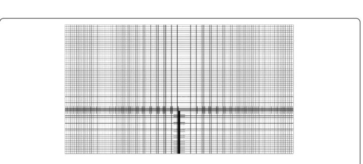
Figure 2 Baseline grid.
The tank has two holes in the upper wall, so that zero pressure can be prescribed there. When D simulations are performed, symmetry boundary conditions are used on the faces with normal in they-direction and no slip conditions are enforced on the remaining walls. When D simulations are performed, no slip is enforced on all walls. The beam is clamped at the point A. When D simulations are performed, all nodes of the solid mesh are locked in they-direction, leading to a plane strain assumption.
Figure 3 Temporal history of the rotation angle.
Figure 4 Volume fraction: blue corresponds toα= 0 (air) and red corresponds toα= 1 (oil).
In the simulations, the gravitation vector was rotated instead of rotating the whole do-main. The centrifugal forces, arising from the fact that the simulation is performed in an accelerating coordinate system, have been neglected. This is justified because the angu-lar velocity of the motion is small. As will be seen, good results are obtained with this approximation.
Four seconds of physical time are simulated, covering three full periods of the beam mo-tion. Figure shows snapshots from a D simulation at different time steps. The angular frequency of the forced rotation is close to the eigenfrequency of the system and there-fore the waves grow larger with time. The beam undergoes large deformation due to the interaction with the fluid.
Figure 5 Tip displacement of a beam in a rolling tank: spatial convergence and comparison with reference data.
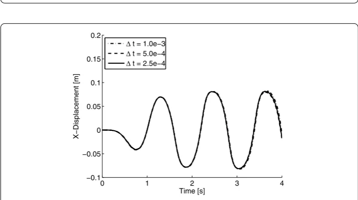
Figure 6 Temporal convergence of tip displacement.
and the simulations in [] is very good. The differences between the results obtained with grid (, fluid cells and solid elements), grid (, fluid cells and solid elements) and grid (, fluid cells and , solid elements) are small, indicating that grid convergence has been obtained. Figure shows the displacement predicted with grid for three different time steps. The differences are small, indicating that the time step is sufficiently short.
Figure 7 Comparison between our simulations and results from the literature.
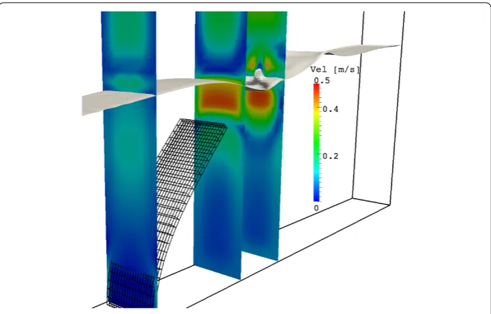
Figure 8 Snapshot from the 3D simulation.The interface and the grid are colored by the fluid velocity and 3D effects are clearly visible on the oil-air interface.
decreasing the amplitude of the motion. This effect is not captured in a D simulation, where symmetry (free slip) boundary conditions are applied to the walls with normal in they-direction. Furthermore, the D simulation captures the small gap between the beam and walls in they-direction. The D effects are clearly visible in Figure , that shows the beam and the oil-air interface. The velocity variations iny-direction due to the walls can be seen in Figure , that shows the velocity magnitude in several planes in the domain.
The D simulations presented in Figure were performed without coupling iterations. However, Gauss-Seidel iterations were used in the D simulation to get a stable solution.
Conclusions
Figure 9 Snapshot from the 3D simulation.The slices are colored by the fluid velocity. The 3D effects induced by the wall can be seen in the oil as well as in the air.
a volume of fluids method. The discretization is performed on an adaptive octree grid allowing grid refinements around the structure and the oil-air interface. By coupling the Navier-Stokes solver with a structural dynamics solver for large deformations a robust framework for three-dimensional fluid-structure interaction applications is realized. The good agreement with previously published data demonstrates the accuracy.
Competing interests
The authors declare that they have no competing interests.
Authors’ contributions
The main idea of this paper was proposed jointly by the authors. ES implemented and designed the structure model, performed the numerical experiments and prepared the first version of the manuscript. AM implemented and designed the fluid model. ES and AM jointly designed and implemented the fluid-structure coupling. All authors read and approved the final manuscript.
Acknowledgements
This work was supported in part by the Sustainable Production Initiative and the Production Area of Advance at Chalmers. The support is gratefully acknowledged.
Received: 30 April 2012 Accepted: 5 March 2014 Published:03 Jun 2014 References
1. Hu H, Patankar N, Zhu M:Direct numerical simulation of fluid-solid systems using arbitrary Lagrangian-Eulerian technique.J. Comput. Phys.2001,169:427-462.
2. Monaghan J:Smoothed particle hydrodynamics.Rep. Prog. Phys.2005,68:1703-1759. 3. Cummins S, Rudman M:An SPH projection method.J. Comput. Phys.1999,152:584-607.
4. Onate E, Idelsohn S, Pin FD, Aubry R:The particle finite element method. An overview.Int. J. Commer. Manag.2004,
1:267-307.
5. Peskin C:Numerical analysis of blood flow in the heart.J. Comput. Phys.1977,25:220-252.
6. Majumdar S, Iaccarino G, Durbin P:RANS solvers with adaptive structured boundary non-conforming grids.
Technical report. Center for Turbulence Research; 2001.
7. Mark A, van Wachem B:Derivation and validation of a novel implicit second-order accurate immersed boundary method.J. Comput. Phys.2008,227:6660-6680.
8. Mark A, Rundqvist R, Edelvik F:Comparison between different immersed boundary conditions for simulation of complex fluid flows.Fluid Dyn. Mater. Proc.2011,7(3):241-258.
9. Mark A, Svenning E, Rundqvist R, Edelvik F, Glatt E, Rief S, Wiegmann A, Fredlund M, Lai R, Martinsson L, Nyman U:
10. Forster C, Wall W, Ramm E:Artificial added mass instabilities in sequential staggered coupling of nonlinear structures and incompressible viscous flows.Comput. Methods Appl. Math.2007,196:1278-1293.
11. Degroote J, Bathe K, Vierendeels J:Performance of a new partitioned procedure versus a monolithic procedure in fluid-structure interaction.Comput. Struct.2009,87:793-801.
12. Doormaal JV, Raithby G:Enhancements of the SIMPLE method for predicting incompressible fluid flows.Numer. Heat Transf.1984,7:147-163.
13. Rhie C, Chow W:Numerical study of the turbulent flow past an airfoil with trailing edge separation.AIAA J.1983,
21:1527-1532.
14. Ubbink O:Numerical prediction of two phase fluid system with sharp interfaces.PhD thesis. Imperial College of Science, Department of Mechanical Engineering; 1997.
15. Mase G:Continuum Mechanics. New York: McGraw-Hill; 1970.
16. Bonet J, Wood R:Nonlinear Continuum Mechanics for Finite Element Analysis. Cambridge: Cambridge University Press; 1997.
17. Belytschko T, Liu W, Moran B:Nonlinear Finite Elements for Continua and Structures. New York: Wiley; 2000. 18. Hughes T:The Finite Element Method. New York: Dover; 1987.
19. Sauer G:Alternative reduced integration avoiding spurious modes for 8-node quadrilateral and 20-node hexahedron finite elements.Forsch. Ingenieurwes.1999,65:131-135.
20. Newmark N:A method of computation for structural dynamics.J. Eng. Mech.1959,85:67-94.
21. Botia-Vera E, Bulian G, Lobovsky L:Three SPH novel benchmark test cases for free surface flows. In5th ERCOFTAC SPHERIC Workshop on SPH Applications; 2010.
22. SPHERCIC benchmarks. [http://canal.etsin.upm.es/ftp/SPHERIC_BENCHMARKS/]
23. Degroote J, Souto-Iglesias A, van Paepegem W, Annerel S, Bruggeman P, Vierendeels J:Partitioned simulation of the interaction between an elastic structure and free surface flow.Comput. Methods Appl. Math.2010,199:2085-2098.
10.1186/2190-5983-4-7