R E S E A R C H
Open Access
Focal plane model for flat refractive
geometry
Garrett W. Mann
1*and Steven J. Eckels
2Abstract
Background: Flow visualization techniques such as uPIV and droplet imaging determine the measurement volume by the focal plane. Thus, an understanding of how the focal plane moves in reference to the camera is necessary when planar interfaces are present between the camera and the focal plane.
Methods: Using geometric optics, a focus model for a camera imaging through multiple parallel interfaces with different refractive indices is derived. This model is based on the thin lens camera model and gives the location of the focal plane, the depth of field, and the change in the location of the focal plane for a change of camera position. The theoretical model is validated by both simulation and experimental results.
Results: Significant results are that while the magnification of a camera for an in-focus object does not vary for changes in the camera position, the position of the focal plane does. The change of the focal plane location depends only on the refractive indices of the media surrounding the camera and the focal plane regardless of the number or type of other media in between.
Conclusion: The derived model provides a simple, accurate relationship between the focal plane location and the number and location of planar interfaces, thus avoiding potentially incorrect results for measurement plane depth.
Keywords: Focal plane, PIV, Refractive geometry, Depth of field
Background
Particle image velocimetry (PIV) is one of the most prominent measurement techniques for full-field flow quantification. Of particular recent interest, with the rise of micro-electromechanical systems (MEMS) technology and microfluidics, is the field ofμPIV—measuring veloc-ity fields of small channel flows at high magnification (see [1] for a review). Various challenges arise when apply-ing this technique to small scales, includapply-ing diffraction effects, errors due to Brownian motion and spurious reflections, and the necessity of setting the measurement volume using the depth of field instead of light sheet thickness. The latter of these challenges shifts the respon-sibility of accurately locating the measurement volume to the imaging rather than light sheet optics. Thus, the measurement volume location and thickness are deter-mined by the parameters of the camera and lens combi-nation such as numerical aperture (NA), focal length, and
*Correspondence: [email protected]
1Mann Engineering Consulting, 115 Carnegie Pl., 15208 Pittsburgh, PA, USA Full list of author information is available at the end of the article
magnification. The thickness of the measurement volume for volume-illuminatedμPIV has been thoroughly stud-ied. Meinhart et al. [2] derived the depth of measurement volume accounting for diffraction, geometric optics, and particle size. Olsen and Adrian [3] derived the depth of correlation for the measurement volume—the thickness outside of which a particle does not make a significant contribution to the cross-correlation of the interrogation regions. On the other hand, very little has been said about the location of the focal plane. Both of these considera-tions become more complicated when multiple interfaces are situated between the camera and the focal plane (e.g. the camera views through a window into a medium other than air), which is a common situation in μPIV applications.
For the macro-scale PIV case, various models have been proposed to correct the distortions from such changes of optical media. Wieneke proposed a self-calibration scheme where the location of the laser light sheet was inferred without a calibration target using the dispar-ity map from de-warped images from two stereoscopic
cameras [4]. He showed that the Tsai pin hole camera model [5] could accurately model the distortion induced by the planar interface, although the parameters of the model no longer took on physical values. For his proposed self-calibration scheme when the camera system was ini-tially calibrated in air and then self-calibrated in water, he proposed the three interface model of Maas [6] and was able to accurately self-calibrate as long as the distance and misalignment between the window and the light sheet could otherwise be accurately inferred. He also verified that using Tsai’s model along with Maas’ three interface model allowed the Tsai intrinsic parameters to assume physically realistic values.
For applications other than PIV, such as underwater photography and photogrammetry, several models and calibration techniques have been proposed to explicitly correct for the distortion due to a change of refractive media. Kwon proposed a modification of the direct linear transform (DLT) model using Snell’s law to explicitly cor-rect for this [7, 8]. Simulations using this model showed a significantly smaller error than the DLT model. How-ever, his calibration method required the prior knowledge of the location and orientation of the planar interface. Treibitz et al. show that a camera viewing a scene through multiple refractive geometry is not a single viewpoint sys-tem [9]. They proposed a camera calibration method for estimating the focal length of the camera and the distance from the camera center to the interface based on mini-mizing the length in the world space of a known straight object. Agrawal et al. further extended this area, show-ing the system is essentially an axial camera [10]. They proposed a calibration method based on 2D-3D point cor-respondences where the 3D calibration points have an unknown pose. The calibration scheme allows them to estimate the orientation of the camera with respect to the interfaces, the thicknesses of the interfaces, and the indices of refraction.
However, none of these models address the effect of multiple refractive geometry on the location of the focal plane or the depth of the measurement volume. While effects of refractive geometry are perhaps understood by the community (e.g. Meinhart et al. [2] mention adjusting the movement of a microscope by the ratio of the refrac-tive indices), the authors are not aware of an organized exposition of these effects and their practical implica-tions anywhere in the literature. Thus, there is warrant for revisiting this topic to provide better clarity for further research in the area ofμPIV and other experimental flow visualization methods.
Therefore, this paper presents the relationship between the location of the focal plane and the orientation of the camera with respect tomparallel planar index of refrac-tion changes using a first order geometric model. This relationship is demonstrated without complicated optical
theory to make the results usable to experimentalists from domains other than optics. The model is an extension of the thin lens, paraxial model and is derived for the case where the optical axis is perpendicular to the planar interfaces.
Methods
Model development
A thin lens is described by two idealizations. First, all rays traced through the lens are assumed to be close enough to the optical axis so that the trigonometric functions of the angle between the ray and the axis can be approximated accurately with a first order Taylor series expansion. Sec-ond, the thickness of the lens is small enough that the two principle planes of the lens are assumed to be superim-posed. Thus, a ray intersecting the center of the lens at the optical axis will continue in the same direction with-out deviation. These two assumptions ensure that all rays from object points will intersect at a single image point, and thus the thin lens model can exactly describe a pinhole camera model. However, the additional parameter—the distance of the image plane from the camera center, allows information about focus to be inferred. For many imag-ing scenarios, the thin lens assumptions are justified the distance of the object to the camera is large compared to the size of the aperture. Additionally, most modern optical systems are designed to minimize the aberrations caused by the limitations in this model.
In this paper, the thin lens model will be extended to include the effect of multiple parallel interfaces between the camera and the focal plane. The analytical expres-sions regarding the focal plane location will be derived using the paraxial assumption for the rays passing through the planar interfaces as well as through the thin lens.
Figure 1 shows a ray leaving an object, passing through the parallel interfaces, and being focused by the thin lens to potentially form an image on the image plane. Under the paraxial assumption, an arbitrary ray passing through a thin lens may be considered to continue directly to the principle plane and be bent according to the relation [11]
θ=θ+yφ, (1)
whereθandθare the small angle between the ray and the normal to the principle plane for the entering and leaving ray respectively (a ray with a positive slope has a posi-tive angle),yis the height above the optical axis where the ray intersects the principle plane, andφ is the power of the refracting system, which is the reciprocal of the focal length of the lens or 1/f.
Fig. 1Ray tracing diagram for focal plane model withmchanges in index of refraction
Fig. 1, the height where the ray hits the principle plane of the lens is
y0=h0−
m
i=0
ziθi, (2)
where the small angle approximation tan(θi) ≈ θi has been used. The negative sign comes from the sign conven-tion assumed for the slope of the ray: the angle that the ray makes with the interface is positive if the slope of the ray is positive with respect to the camera coordinate system. For positive ray slopes with respect to the coordinate sys-tem, the intersection point of the ray with a surface closer to the origin will be lower.
Snell’s Law can be used to writeθiin terms ofθmand the refractive indices. By applying Snell’s Law, in first order, recursively at each interface, theith angle is given as
θi=
nm
ni
θm. (3)
Thus, the angle of the ray where it hits the principle plane of the lens is
θ0= nm
n0
θm. (4)
and the height of this point is given by
y0=hO− m
i=0
zi
nm
ni
θm. (5)
The ray is then bent by the lens according to Eq. (1) so that the new angle is
θI=
nm
n0
θm+
hO−
m
i=0
zi nm ni θm 1
f. (6)
Because of the paraxial assumption, this angle is the same as the slope of the ray forming the image. Thus the
image height can be expressed as a linear equation inz
whereθIis the slope andy0is the intercept,
hI(z,θm)=
nm
n0
θm+
hO−
m
i=0
zi nm ni θm 1 f
z+hO
−
m
i=0
zi
nm
ni θm.
(7)
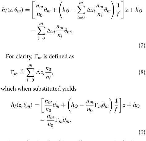
For clarity,mis defined as
m
m
i=0
zi
n0 ni
, (8)
which when substituted yields
hI(z,θm)=
nm
n0
θm+
hO−
nm
n0
mθm 1
f
z+hO
− nm
n0
mθm.
(9)
Any ray leaving the object will create a ray in the image space with a height given by this equation. Any two rays leaving the object will intersect to form an image point. By solving for the image point using two arbitrary rays, it can be shown that all rays leaving the object point and captured by the lens will intersect to form a single image point. The rays will be distinguished by the angles leaving the object pointθmandθm. The system is
hI=
nm
n0
θm+
hO−
nm
n0
mθm 1
f
z+hO−
nm
n0
mθm
(10)
hI=
nm
n0
θm +
hO−
nm
n0
mθm 1
f
z+hO−
nm
n0
mθm .
Solving forzandhIyields
z= mf f −m
(12)
and
hI =
hOf
f −m
. (13)
Note that neither of these expressions depend on the value of θ or θ. Thus, all rays leaving an object and captured by the lens intersect at a single image point.
LetdIbe the distance of the image plane from the prin-ciple point (e.g.z). From Eq. (12),mcan be expressed as
m= dIf
dI−f
. (14)
Using the definition ofm, the distance from the final interface to the object plane is
zm=
nm
n0
dIf
dI−f − m−1
i=0
zi
n0 ni
. (15)
This result is almost the same as a thin lens by itself, and it simplifies to this as the indices of refraction converge. The difference is that the distance from the camera to the object is modified by the ratios of refractive indices of the different segments.
Using this expression, the movement of the focal plane location with changes in camera location can be demon-strated. For image measurement techniques, it is critical to be able to evaluate this relationship in order to record data from the proper slice of a flow. First consider from Eq. (15) that the location of the focal plane with respect to themth interface is a function ofz0. Thus an
incremen-tal change inz0will lead to a differential change inzm. Expressly,
δzm=zm(z0−δz0)−zm(z0) (16)
A negative differential change indicated in Eq. (16) cor-responds to the camera moving towards the interfaces. Using Eq. (15),δzmis equivalent simply to
δzm=
nm
n0
δz0 (17)
Simulations
In the above derivations, the paraxial assumption was made for the rays passing through the refractive planes. This is only a reasonable assumption for object points close to the optical axis at a sufficient distance from the lens. Thus, it is important to validate this assumption by simulating the full physics of the rays for typical opti-cal systems to see how the full solution differs from the approximation. Without the paraxial assumption at the
parallel interfaces, the expression for the image height can be shown to be, using the same nomenclature as in Fig. 1,
hI(z)=
⎡ ⎢ ⎢ ⎣
nm n0 sin(θm)
1−
nm n0
2
sin2(θm) + y0
f ⎤ ⎥ ⎥
⎦z+y0, (18)
where y0 is the height of the ray where it intersects the
principle plane of the lens and is given by
y0=hO− m
i=0
zisin(θm)nmni
1−
nm ni
2
sin(θm)2
, (19)
and where θm is the angle between the ray leaving the object point and the optical axis. In general, there is no image point that is common to all rays leaving the object under this model.
Because of this, focus information must be inferred by finding the location of the image plane that results in the least blur of the image. This location was computed using the envelope of the curve (caustic) formed by Eq. (18) for all rays captured by the camera. The intersection points of this envelope with the rays passing through the aperture limits on the top and bottom of the lens gave the likely locations of the smallest bundle of rays. For the simula-tion, these intersection points were solved for numerically and all possible combinations were computed to find the image location for the smallest bundle.
Table 1Simulation results forμPIV case
NA hO/FOV zmFull zmParaxial δzmFull δzmParaxial
0.05 0 2.000 1.9991 0.1996 0.1995
0.10 0 2.000 1.9964 0.1997 0.1995
0.20 0 2.000 1.9859 0.2004 0.1995
0.05 0.25 2.000 1.9986 0.1996 0.1995
0.10 0.25 2.000 1.9954 0.1998 0.1995
0.20 0.25 2.000 1.9839 0.2005 0.1995
0.05 0.50 2.000 1.9977 0.1996 0.1995
0.10 0.50 2.000 1.9942 0.1999 0.1995
0.20 0.50 2.000 1.9818 0.2005 0.1995
towards the interfaces. Table 2 gives the results of the simulation.
In both of these simulations, the accuracy of the first order model decreases as the object height and aperture increases. However, even at the largest aperture and object height, the relative error between the full model and the paraxial model is less than 1% indicating that the first-order model can be accurately be used for these imaging situations. However, as indicated by the simulations, the error induced by this approximation increases with FOV and aperture. Imaging setups with FOV or aperture much larger than those used in the above simulations could result in significant errors.
Experimental validation
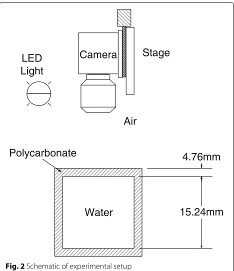
The model was validated by performing experiments on a long distanceμPIV setup. Figure 2 gives a schematic for the experimental facility. The camera was mounted over a square polycarbonate duct with a copper bot-tom. A 25 μm [0.001in] resolution stage was used to move the camera with respect to the camera interface. Water was circulated in the duct. Light was supplied by means of an LED lamp. The camera used for the
experi-Table 2Simulation results for droplet imaging case
f-stop hO/zi zmFull zmParaxial δzmFull δzmParaxial
f/32 0 33.3375 33.3374 10.1972 10.1972
f/11 0 33.3375 33.3374 10.1972 10.1972
f/2.8 0 33.3375 33.3374 10.1972 10.1972
f/32 0.25 33.3375 33.3136 10.1972 10.1977
f/11 0.25 33.3375 33.3136 10.1972 10.1977
f/2.8 0.25 33.3375 33.3136 10.1972 10.1977
f/32 0.50 33.3375 33.2252 10.1972 10.1994
f/11 0.50 33.3375 33.2252 10.1972 10.1994
f/2.8 0.50 33.3375 33.2252 10.1972 10.1994
15.24mm Water
Air Camera
Polycarbonate LED
Light
4.76mm Stage
Fig. 2Schematic of experimental setup
ments was a machine vision camera (TSI PowerView Plus 4 MP) with a long distance microscope (K2/SC Infinity with CF-4).
The procedure of the experiment was as follows:
1. The camera was focused on the outside of the polycarbonate duct using the focus adjustment on the K2 lens.
2. A focused image of the top of the polycarbonate was captured.
3. Using the traverse, the camera was moved towards the duct until the bottom surface of the
polycarbonate wall was in focus. The displacement required was recorded, and an image was captured. 4. The camera was then lowered until the bottom of the
duct was in-focus. The displacement required was recorded and an image was captured.
Figure 3 shows the focused images of the top, bottom of top wall, and bottom of duct locations. The measured displacements of the camera required to achieve these sharp images in comparison to the model are shown in Table 3. The indices of refraction for air, polycarbon-ate, and water were assumed to be n = 1.0, n = 1.6, andn=1.33.
a
b
c
Fig. 3Images taken during experiments.aTop of duct (outside),bTop of duct (inside),cBottom of duct
Results and discussion
From this focus model, the location of the focal plane, implications about the magnification of the system, and how these factors change with movement of the camera or for different orientations of the planar interfaces can be inferred.
Location of focal plane
From Eqs. (14) and (17), several important conclusions can be derived. First, movement of the camera will not produce equal movement of the focal plane unless
nm
n0 = 1. Secondly, the amplification of the motion of the camera does not depend on the location of the focal plane. Thus, Eq. (17) holds regardless of the location of the camera with respect to the interface. Also from these equations, the only factor that affects this relationship is the refractive indices of the media surrounding the lens and the focal plane. Thus, the number or type of media changes in between the camera and the focal plane have no effect on the relationship between camera and focal plane movement.
A more complete understanding of this result can be seen by realizing that the right hand side of Eq. (14) only depends on the type and adjustment of the lens. Thus, if the focus adjustment of the lens remains fixed, m is constant, despite the number of interfaces, the indices of refraction, or the relative location of the camera to the interfaces changing. If the optical system has been focused on a known location to determine the left hand side of Eq. (14), any of the parameters of the left hand side can
Table 3Experimental results
Level Geometric Model-predicted Actual camera Diff (%) location camera motion motion (mm)
(mm) (mm)
Top of duct 0 — — —
Bottom of top wall
4.76 2.98 2.94 -1.2%
Bottom of duct
20.00 14.44 14.20 -1.7%
be solved for after a change in the location or type of the interfaces.
Magnification of image
From the results in Eq. (13) immediately follows that the magnification of the system is
M hI hO =
f
f −m. (20)
The magnification written in terms of the distance to the image,dI−zfrom Eq. (12) is
M= f −dI
f . (21)
Note that here the magnification is defined to be negative if the image is inverted.
Equation (21) is identical to the magnification of a sin-gle thin lens [11]. However, Eq. (20) is different. This leads to the important conclusion that, from the perspective of the camera, the magnification of the image is not changed by the insertion of the refractive interfaces. However, the location where the camera is in focus and where the mag-nification holds, does change. For example, consider a camera that is focused on an object in air. If a window is placed between the object and the camera and the space surrounding the object filled with water, the location of the center of the focal plane would no longer be at the object. However, if the object was moved to the new loca-tion of the focal plane, the magnificaloca-tion would be the same as before the window was put in place. If instead the camera was re-focused on the current location of the object after the insertion of the window, the magnification would change according to how the re-focusing changes
dIin Eq. (21).
Conclusions
In this paper, a first order, geometrical optics focus model for a camera looking through multiple planar interfaces was presented. The model demonstrates the following relationships between the object focal plane and the ori-entation of the camera to the planar interfaces:
1. For fixed focus, the magnification of the camera is not changed by the addition or removal of planar interfaces between the camera and the object; however, the location of the focal plane where that magnification holds, does change.
2. Motion of the camera towards or away from the refractive interfaces results in a movement of the focal plane of the camera that is magnified by the ratio of the refractive indices of the media surrounding the object and the camera regardless of the number or type of media between the object and the camera. 3. For a fixed lens focus, the optical path length
between the camera center and the focal plane is fixed regardless of changes in number of interfaces, index of refraction, or relative location of the camera to the interfaces.
The paraxial assumption of the model has been vali-dated for typical imaging cases through simulation, and the main consequences of the model have been validated experimentally.
Abbreviations
DLT: Direct linear transform; FOV: Field of view; MEMS: Micro-electromechanical machines; NA: Numerical aperture; PIV: Particle image velocimetry
Acknowledgements
None
Funding
This project was internally funded by the Institute for Environmental Research.
Availability of data and materials
The dataset supporting the conclusions of this article is included within the article.
Authors’ contributions
GWM performed the analysis and was the lead author of the manuscript. SJE developed the experimental program and suggested the final presentation of the results. Both authors read and approved the final manuscript.
Competing interests
The authors declare that they have no competing interests.
Publisher’s Note
Springer Nature remains neutral with regard to jurisdictional claims in published maps and institutional affiliations.
Author details
1Mann Engineering Consulting, 115 Carnegie Pl., 15208 Pittsburgh, PA, USA. 2Institute for Environmental Research, Kansas State University, 920 N. 17th St., 56 Seaton Hall, 66506 Manhattan, KS, USA.
Received: 5 October 2017 Accepted: 20 November 2017
References
1. Lindken, R, Rossi, M, Große, S, Westerweel, J: Micro-particle image velocimetry (μpiv): recent developments, applications, and guidelines. Lab Chip.9(17), 2551–67 (2009)
2. Meinhart, C, Wereley, S, Gray, M: Volume illumination for two-dimensional particle image velocimetry. Meas. Sci. Technol.11(6), 809 (2000) 3. Olsen, M, Adrian, R: Out-of-focus effects on particle image visibility and
correlation in microscopic particle image velocimetry. Exp. Fluids.29(1), 166–174 (2000)
4. Wieneke, B: Stereo-piv using self-calibration on particle images. Exp. Fluids.39(2), 267–280 (2005)
5. Tsai, RY: A versatile camera calibration technique for high-accuracy 3d machine vision metrology using off-the-shelf TV cameras and lenses. IEEE J. Robot. Autom.3(4), 323–344 (1987)
6. Maas, H-G: Contributions of digital photogrammetry to 3-D PTV. In: Three-Dimensional Velocity and Vorticity Measuring and Image Analysis Techniques, pp. 191–207. Springer, Berlin, (1996)
7. Kwon, Y: A camera calibration algorithm for the underwater motion analysis. In: ISBS-Conference Proceedings Archive, vol. 1. University of Konstanz, Konstanz (1999)
8. Kwon, Y, Casebolt, JB: Effects of light refraction on the accuracy of camera calibration and reconstruction in underwater motion analysis. Sports Biomech.5(2), 315–340 (2006)
9. Treibitz, T, Schechner, YY, Kunz, C, Singh, H: Flat refractive geometry. IEEE Trans. Pattern Anal. Mach. Intell.34(1), 51–65 (2012)
10. Agrawal, A, Ramalingam, S, Taguchi, Y, Chari, V: A theory of multi-layer flat refractive geometry. In: Computer Vision and Pattern Recognition (CVPR), 2012 IEEE Conference On, pp. 3346–53. IEEE, New York (2012)