April 6, 16, 28, 2015
The Ideal of the Completeness of Calculi of Inductive Inference: An
Introductory Guide to its Failure
John D. Norton1
Department of History and Philosophy of Science Center for Philosophy of Science
University of Pittsburgh http://www.pitt.edu/~jdnorton
Non-trivial calculi of inductive inference are incomplete. This result is demonstrated formally elsewhere (Norton, manuscript). Here the significance and background to the result is described. This note explains what is meant by incompleteness, why it is desirable, if only it could be secured, and it gives some indication of the arguments needed to establish its failure. The discussion will be informal, using illustrative examples rather than general results. Technical details and general proofs are presented in Norton (manuscript).
Introduction
The first part of this paper describes what it would be for a calculus of inductive inference to be complete, using the illustration of the Bayesian analysis of simplicity; and it explains why the completeness is desirable, if only it could be secured. In brief, completeness is achieved when computations in the calculus are carried out in a domain sufficiently large so that the computations do not need to call upon inductive content that is external to the domain.
Completeness would allow us to characterize inductive inference merely as inference that
conforms to the calculus at issue. This characterization would provide a clear and simple solution to the enduring foundational problems of inductive inference. All such problems would be
reduced to questions answerable by computation in the calculus.
This attractive solution to the foundational problems fails. Non-trivial calculi of inductive inference are incomplete. These incomplete calculi include many more than just the probability calculus. This incompleteness explains why particular calculi of inductive inference are beset by lingering difficulties. The Bayesian system is perpetually struggling to overcome the problem of the priors. Augmented calculi are repeatedly proposed to solve problems in older calculi, while none manages without its own, new problems. All these problems arise because we are really trying to formulate a complete calculus of inductive inference. That they must linger unsolved does not derive from a failure of our imagination to hit upon just the right solution. It is a necessity derived from incompleteness.
The second part of this paper will provide a simplified guide to the full proof of this failure, given elsewhere. Here is a terse summary of the main result that will be introduced and explained in greater detail in this paper. The incompleteness arises from the combination of two desirable properties of calculi of inductive inference.
The first property is an expression of completeness: we can find a sufficiently large set of propositions in which the inductive strengths of support are fixed by relations in the set, without the need to import any inductive content from outside it. Since the only other inferential
resources within the set are the deductive relations among the propositions, this amounts to requiring that the inductive strengths of support are fixed by the deductive relations among the propositions in the set. This requirement is unremarkable. The Kolmogorov axioms of
probability theory are a routine part of such a specification. These axioms adapt the probabilities to the deductive structure. They need only a small supplement to fix the probabilities uniquely.
The second property involves disjunctive refinements of propositions. Through them we replace a proposition
“Person X is in Boston.” by a disjunction of its disjunctive parts:
Such disjunctive refinement increases the expressive power of the set of propositions and leads to adjustments of the inductive strengths of support. The requirement of asymptotic stability asserts that continuing disjunctive refinement eventually provides such diminished further power that the inductive strengths of support among some fixed set of propositions stabilize to limiting values. Further refinement eventually becomes inert, inductive hair-splitting.
The failure of the completeness resides in the impossibility of sustaining both properties.2 In briefest terms, the deductive closure of any set of propositions is highly symmetric. Each of the non-contradictory, logically strongest propositions—the “atoms”—enter into the same deductive relations. As a result, a deductively definable logic of induction must treat them alike. Each new disjunctive refinement will alter the atoms and, as a result, the inductive strengths throughout the set. It turns out that a deductively definable logic of induction will continue to respond without stabilization to suitably crafted, continuing disjunctive refinements, unless it is a trivial logic that assigns the same limiting inductive strengths everywhere.
One might be tempted by an obvious rejoinder: if continuing refinement causes
continuing problems, stop refining! Declare one specific refinement as preferred; or declare that its propositions comprise a preferred language. That resolves the problem. But the decision of when to stop or which is the preferred language must be made on external, inductive grounds. It privileges certain propositions and thus amounts to the introduction of external inductive content, in violation of the requirement of completeness.
The third part of this paper takes stock and reviews possible responses.
PART I. The Ideal of Completeness
The Many Problems of Induction
Philosophical accounts of inductive inference are not in good shape. Simple enumerative induction fails more than it succeeds. It is almostnever the case that, when some As are B, it also happens that all As are B. Other approaches embroil us in larger philosophical puzzles with little
hope of resolution. Infer to the best explanation, we are told. But we are offered no precise characterization of just what is a good explanation or why explaining, whatever it is, has such evidential powers. Ad hoc hypotheses do not deserve evidential support, we are told. But we are left to wonder why an hypothesis is punished for being tailored to fit the evidence. Is not that sort of fit just what we seek? Finally, to mention an example that will return below, evidence favors simpler hypotheses, we are told. But we have no serviceable characterization of what makes an hypothesis simpler or why such hypotheses should be favored.
These are just the beginnings of the difficulties. Over the centuries, inductive inference has attracted a fulsome collection of general problems that threaten the very cogency of this form of inference. We have Hume’s problem, Hempel’s raven, Goodman’s grue and Quine’s
underdetermination. The difficulties are so enduring that mere mention of induction calls philosophical pain to mind.
Calculating Mechanically
The tenacity of these problems stands in striking contrast with deductive inference. While there are always complications at the fringes, the core is stable to the point of tedium. Modus ponens is a valid argument. Affirming the consequent is a fallacy. These facts of logic leave no room for doubt or debate. We separate the valid from the invalid deductive inferences merely by checking whether the argument form used is one of the approved argument forms in a logic textbook. The exercise is reminiscent of making travel plans by checking a train timetable.
In this regard, deductive logic is more like arithmetic than inductive inference. It is an uncontested, particular fact of arithmetic that 7,919 is the thousandth prime number; and it is merely a matter of tedious computation using standard algorithms to check it. More general facts have a similar security. That there are infinitely many prime numbers is proved by a theorem known since the time of Euclid. Anyone who doubts the infinity of the primes can consult the proof and, by working through its steps, receive all the assurance a reasonable person could require.
A Calculus for Inductive Inference?
puzzles of induction be converted into queries that can be put to and answered by mechanical computation in some suitable calculus? The presently most popular approach to inductive inference, the Bayesian approach, holds out the promise of such a solution. The approach is based on the supposition that inductive support or warranted belief is captured by the mathematical calculus of probabilities. Much of Bayesian analysis is the tedious working of proofs in the calculus. The strength of inductive support provided by some item of evidence for some hypothesis is computed numerically as a conditional probability. General facts about inductive inference are established as theorems of the probability calculus, much as Euclid proved the infinity of the primes. In each case, we have the comforting assurance that, one way or another, a computation will provide a precise answer to our question.
A Bayesian Analysis of Simplicity
Here is an illustration of such a computation. A familiar principle is that evidence favors a simpler hypothesis. For example, when we fit a curve to data, we may find a good enough fit from the hypothesis of a straight line and a slightly better fit from a parabola. We are routinely willing to forgo a slightly better fit by a parabola for the lesser fit of straight line, because we prefer to use the simpler hypothesis.
This preference for the simpler can be vindicated in Bayesian analysis. The key to it is that there are fewer of the simpler hypotheses. A straight line—“y=ax+b”—is fixed by just two adjustable parameters, a and b. A parabola—“y=ax2+bx+c”—is fixed by three parameters, a, b and c. Hence there are many more of the more complicated hypotheses. The straight line hypotheses form a two dimensional space. The parabolic hypotheses form a three dimensional space.
A still simpler example uses this fact and will suffice to get to the key point. Imagine that we have to choose between a simple hypothesis and a more complicated one. Let us say that the simple hypotheses is drawn from a ten-membered set {Hsim1, Hsim2, … , Hsim10} of hypotheses of comparable simplicity. The complicated hypothesis is drawn from a much larger,
one-hundred-membered set {Hcom1, Hcom2, … , Hcom100} of hypotheses of comparable complication. We shall assign equal prior probability to each set:
where conditionalization on a background Ω is supposed but not represented. We then spread the probability uniformly within each set. Since the second set has ten times as many members as the first, the prior probability of any of individual simple hypothesis Hsim i is ten times as great as the prior probability of any of the complicated hypotheses Hcom k.
€
P(Hsimi)
P(Hcom k)
=10 (2) Let us say that the two hypotheses Hsim i and Hcom k fit roughly equally well with the evidence. That is, the supposition of each makes the evidence E roughly equally probable:
P(E|Hsim i) ≈ P(E|Hcom k)
so that the ratio of likelihoods P(E|Hsim i) / P(E|Hcom k) ≈ 1. The relative strength of support from the evidence and background together for the hypotheses is expressed by the ratio of posterior probabilities P(Hsim i|E) / P(Hcom k|E). It can be calculated with the ratio form of Bayes’ theorem:
€
P(Hsim i|E) P(Hcom k|E)
= P(E|Hsimi) P(E|Hcom k)
⋅ P(Hsim i)
P(Hcom k)
Since the likelihood ratio is approximately one, the ratio of the priors (2) is the deciding factor that gives a large boost to the probability of the simpler hypotheses:
€
P(Hsimi|E)
P(Hcom k|E)
≈ P(Hsim i) P(Hcom k)
=10 (3) In brief, since there are fewer simpler hypotheses, a natural spreading of prior probabilities (1) can assign higher prior probability to the simpler hypotheses. When the evidence is equivocal in choosing among the hypothesis, this higher prior probability gives the simpler hypothesis the decisive advantage.
both then exponentially penalize the prior probability of each complexity class so that the probabilities can sum to unity.
External Inductive Content
In many examples like this, Bayesian analysis has been able to reduce an inductive puzzle to a computation in the probability calculus. In each case, however, it turns out that the analysis is not self-contained. Each requires supplement by external inductive content. That is, the computation depends on direct or indirect specification of inductive strengths of support by considerations external to the computation.
Take the case of the analysis of simplicity above. We assigned equal probability to the two complexity classes in (1) and then spread the assigned probability uniformly within each class. The outcome was that each of the simpler hypotheses was assigned a greater prior probability; and this was key to the whole analysis. Yet nothing within the probabilistic computation forced this assignment. We could merely have assigned the same prior probability to each hypothesis individually
P(Hsim1) = P(Hsim2) = … = P(Hsim10})
= P(Hcom1) = P(Hcom2) = … =P(Hcom100) (1’) This alternative assignment would have defeated the analysis. For then, instead of (2), we would have had:
€
P(Hsim i) P(Hcom k)
=1 (2’) and the simpler hypothesis would have received no probabilistic boost:
€
P(Hsim i|E)
P(Hcom k|E)
≈ P(Hsimi) P(Hcom k)
=1 (3’) The point is not that the assignment of (1) is unjustifiable. One could certainly conceive circumstances in which we would be warranted in assigning a higher prior probability to a simpler hypothesis. And we could conceive others in which this might not be so.
the assignments of probability in (1) or (1’).
The Ideal of Completeness
A natural response to the presence of the external inductive content in the Bayesian analysis of simplicity is that we have set our boundaries too narrowly. That the simpler hypotheses ought to be assigned a higher prior probability is something that can in turn be learned inductively. In Jeffreys’ analysis of simplicity, we are to assume that nature favors curves drawn from the simpler of his complexity classes. In Solomonoff’s analysis, we are to assume that nature favors hypotheses that are algorithmically simpler. Neither of these are a priori truths. They are contingent facts about the world. Ascertaining their truth is a matter of further inductive investigation. If we extend the boundaries of our computation, we would hope to capture those considerations as well.
What if those considerations in turn depend upon further external inductive content? We would then extend our boundaries still further. Let us suppose that it is possible to extend the boundary of the computational domain so far that no external inductive content is needed. What would result is an account of all the relations of inductive support within the domain that is fully contained in a single, enormous computation in the probability calculus.
While such an enormous computation would surely outstrip any human powers of comprehension, its possibility in principle is of profound foundational importance. It would mean that the probability calculus is all we need for a full understanding of inductive inference within a suitably large domain.
All particular facts of inductive support within that domain would be expressible by
particular probabilistic relations among its propositions. That the straight-line hypothesis is better supported by the evidence would be expressed by its greater probability; and so on for every other particular fact of inductive support.
general, could be known without drawing upon any inductive content from outside the domain. The analysis would be self-contained.
Its Failure
What is shown in Norton (manuscript) and will be reviewed below is that this ideal of completeness is unattainable. A very large class of possible calculi that likely includes any calculus one might realistically consider, proves unable to support this ideal of completeness. This failure is profound foundationally. It tells us something important about the nature of inductive inference itself: it cannot be fully characterized merely by a calculus.
To get a sense of this import, it is helpful to compare it with the familiar incompleteness of arithmetic. It was once quite reasonable to expect that all the truths of arithmetic could be
captured by a few axioms. For example, Peano’s axioms lay down a few simple properties of natural numbers: 1 is a number; every number has a unique successor; and so on. We would hope that we could identify all of arithmetic with all the truths that can be deduced from these axioms.
Famously, Gödel demonstrated that no finite axiom system can capture all arithmetic truths in this way. The truths of arithmetic are something more than what can be deduced from any fixed, finite system of axioms. We may, of course, be able to derive very many important and interesting arithmetic truths from our favorite axiom system. However, no matter which finite axiom system we favor, there will always be arithmetic truths that are external to its theorems.
I hesitate to draw a comparison with Gödel’s result, for his result is profound and his methods extraordinarily ingenious. The corresponding methods for inductive calculi are simple and mechanical and the result rather banal. But the significance of the result for inductive logic is comparable.
PART II. Demonstrating the Failure
Deductive Structure
How is the incompleteness demonstrated? The first step is to fix the environment in which the inductive logic is applied. We take a fixed set of propositions
{A1, A2, … , Am}.
and our concern will be to determine the inductive relations prevailing among these propositions. This set is intended to be not just large, but very large. It might be all the hypotheses entertained in science, all the evidence statements that may support them and every other proposition that in some way mediates between them. That set—all the propositions we have entertained in
science—will be large. But it will still be finite. For there have only been finitely many scientists and, given some finite limit of the length of sentences, only finitely many propositions
expressible.
These propositions come with a deductive structure. That structure is just the set of all deductive entailment relations among the m propositions. It may turn out, for example, that A1235 deductively entails A441; or that A57 and A103 logically incompatible, so that their
conjunction entails the contradiction ∅. The deductive structure is the totality of these deductive relations.
It will be essential for what follows to see that this structure is highly symmetric. That symmetry is harder to see if we consider merely the propositions A1, A2, … , Am by themselves. Rather we take the larger set of propositions generated by Boolean operations; that is, by taking all negations (“not” ~), disjunctions (“or” v) and conjunctions (“and” &) of the propositions. The set of sentences that results is infinite. However the set of logically distinct propositions is not. The set contains many logically equivalent sentences. The sentence A1, for example, is logically equivalent to all of ~~ A1, ~~~~ A1, A1v A1, A1& (A2v~ A2), etc.
A Boolean Algebra of Propositions
finite set of propositions can support only finitely many atoms. Take the simple case of two propositions in the set {A,B}, where we assume they are logically compatible and do not exhaust the space. Then there are four distinct atoms:
a1 = A&B a2 = A&~B a3 = ~A&B a4 = ~A&~B
The proposition a1 is an atom since nothing (other than the contradiction ∅) entails it.
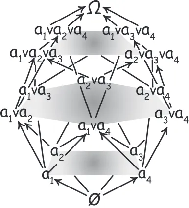
These four atoms generate a four-atom Boolean algebra of finitely many propositions, which has five distinct logical levels
the universal proposition:Ω4 = a1 v a2 v a3 v a4
three-atom disjunctions: a1 v a2 v a3, a1 v a2 v a4, a1 v a3 v a4, a2 v a3 v a4 two-atom disjunctions: a1 v a2, a1 v a3, a1 v a4, a2 v a3, a2 v a4, a3 v a4 atoms: a1, a2, a3, a4
the contradiction: ∅
The original propositions A and B reside within this Boolean algebra as A = a1 v a2 and B = a1 v a3. Figure 1 is a picture of the algebra, showing the distinct levels. The arrows represent
deductive entailment.
Ø
Ω
a
1a
1va
2va
3a
2va
3a
1va
2a
1va
3a
1va
3va
4a
1va
2va
4a
2va
4a
1va
4a
2va
3va
4a
3va
4a
2a
3a
4Symmetries of Deductive Structure
A Boolean algebra is a highly symmetric structure. Informally speaking, each level is homogeneous. That is, the entire algebra “looks the same” from any proposition we pick in the level. For example, take the two-atom disjunction level of the four-atom algebra. Each
disjunction in it is entailed by two atoms; and each disjunction in the two-atom layer in turn entails just two three-atom disjunctions. The only change, as we move around within one of the levels is the labeling of the atoms that appear in the deductive entailments.
When there are very many atoms in the algebra, the basic structure remains the same. There are now, however, many more levels: the one-atom level, the two-atom level, the three-atom level, and so on for very many more levels. As before, each level in the algebra is homogenous. That is, the algebra looks the same, as far as deductive relations are concerned, from each proposition in the same level.
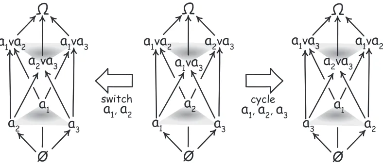
More formally, this symmetry is expressed as a labeling invariance. That is, the total deductive structure is unchanged if we permute the labels attached to the atoms. Take the four atoms
a1, a2, a3, a4
and permute their labels any way you please. You might just switch the first two, so that the atoms are now labeled
a2, a1, a3, a4 Or you might cyclically permute them to
a2, a3, a4, a1
In both cases, propagate the labeling change through the remainder of the algebra. For these permutations and for any others, the total deductive structure will remain unchanged. If a1 entails a1 v a2 entails a1 v a2 v a3 prior to the permutations of atomic labels, the same will be true for the relabeled propositions.
Ø
Ω
a
1a
2va3a
1va
2a
1,a
2 switcha
1cycle, a2, a3a
1va3a
2a
3Ø
Ω
a
1a
2va3a
1va2a
1va
3a
2a
3Ø
Ω
a
1a
2va
3a
1va2a
1va
3a
2a
3Figure 2. Relabelings of a Three-Atom Algebra
Deductively Definable Logics of Induction
A calculus of inductive inference will here be built around the fundamental quantity “[A|B]”, which is the strength of the inductive support afforded proposition A by proposition B. The strength might be a conditional probability, which means that it conforms with the
probability calculus. The strength need not be a probability. It may be a strength that conforms with one of many other calculi.
Other choices are possible for the basic quantity. We could instead use “[A|B,C]”, which could be interpreted as the strength of inductive support afforded proposition A by B with respect to background C. It will become clear that the arguments leading to incompleteness can be mounted in variant form for each of these choices. We will proceed with just [A|B] since it is all that is needed to see how the arguments run.
A calculus of inductive inference is a system of rules that enables the assignment by purely mechanical computation of all the strengths [Ai|Ak] for propositions in the set {A1, A2, … , Am}. They key question is which resources these rules may use. If the domain in which the set resides is sufficiently large for completeness, then the rules may not use any inductive content from outside the domain. That is, it may not set any of the [Ai|Ak] by external considerations independent of the rules of the calculus.
propositions in the larger algebra Ω in which it resides. A calculus that employs just this deductive structure in specifying its strength is “deductively definable.”
Two Sample Logics
At first it may seem that deductive definability is excessively restrictive. It is not. Rather it is the standard way of specifying a calculus of this type. As a general matter, the definitions of the strengths [Ai|Ak] may be supplied by explicit or implicit definitions.
The latter implicit definitions are more commonly used. The celebrated Kolmogorov axioms (1950) for the probability axioms provide implicit definitions solely in terms of the deductive structures among the propositions in the outcome space. These axioms, used to define an additive measure m on the algebra, assert:
For any A, m(A)≥0. (4a)
m(Ω) = 1 (4b)
If A&B=∅, then m(AvB) = m(A) + m(B) (4c)
This is an implicit definition of the additive measure m. It consists of three sentences in which the measure appears; and those sentences otherwise only mention the deductive structure of the algebra. For example, (4b) assigns unity to the universal proposition Ω, distinguished by the fact that it is deductively entailed by all the propositions in the algebra. The summation rule relates the measure of a disjunction to the measures of the disjuncts, in the special case in which the disjuncts are deductively incompatible.
The Kolmogorov axioms constrain the measure m, but do not definite it uniquely. In any given algebra, there will be infinitely many measures compatible with the axioms. We can assure uniqueness of m in some algebra by adding further conditions, such as:
For all atoms, a1, a2, …, an, m(a1) = m(a2) = … = m(an)
(5)
Once again, this sentence mentions only deductive structure. The atoms a1, a2, …, an are the propositions in the algebra that are deductively entailed by no other propositions (other than the contradiction, ∅).
€
[A|B]P =P(A|B)=m(A&B)
m(B) (6) In order to underscore that these results apply to many calculi, we can also define a different calculus—a “specific conditioning” logic—by replacing (6) by the following.3 For all propositions A and B, where neither A nor B is ∅
€
[A|B]SC =P(A|B)=
m(A&B)2
m(A)m(B) (7) We will see shortly in an example what motivates this logic.
General Form of the Definitions
The conditions (4), (5) and (6) implicitly define a probabilistic calculus of inductive inference. The conditions (4), (5) and (7) implicitly define a distinct “specific conditioning” calculus of inductive inference. What will matter in what follows is the general form of the definitions:
General form of the implicit definition:
Set of sentences that mention the strengths [Ai|Ak] and deductive relations among the members of the set {A1, A2, … , Am} and the other
propositions in the algebra.
These two examples are just two of many possible deductively definable logics of induction. More are described in Norton (2010).
A simple and natural one derives from the basic notion of hypothetico-deductive
confirmation. According to it, if hypothesis H deductively entails evidence E, then evidence E inductively supports H. This much provides for a single value “supports” for [H|E] via the explicit definition:
If H deductively entails E, then [H|E] = supports.
There is much scope to enhance the definition. We might replace the single value with increasing numerical values the closer that H is to E in terms of the levels of the Boolean algebra. If, for example, H = a1 v a2 from the level of two atom disjunctions and E = a1 v a2 v a3 v a4 from the
level of four atom disjunctions, then the strength of support might be defined as 2/4. Then the closer they are in levels, the stronger the support. This gives the augmented definition4
If H from the level of m atom disjunctions
deductively entails E from the level of n atom disjunctions, then [H|E] = m/n.
This second example illustrates the general form of an explicit definition of inductive strengths: General form of the explicit definition:
The strengths [Ai|Ak] are determined by a formula that mentions only the deductive relations among the members of the set {A1, A2, … , Am} and the other propositions in the algebra.
In the example, the formula is “m/n”, where the quantities n and m are related to atom counts and are thus recoverable from the deductive structure of the Boolean algebra.
This hypothetico-deductive model could be enhanced still further by rewarding hypotheses with stronger support if they are more explanatory or simpler. To do this requires that we have some way of identifying which hypotheses are more explanatory or which are simpler. If that can be done by adding further propositions to the algebra, then the definition of the inductive
strengths can still meet the requirement that they draw only on resources within the domain. If that cannot be done and these judgments require resources outside the domain, then we have already established that these particular augmentations of the hypothetico-deductive scheme are not complete.
The Quest for an Art Thief
As an illustration, we will imagine an inductive problem presented to the police in their efforts to track down the location of a notorious art thief. They know, we shall say, that the art thief is in one of four cities: Boston “BOS”, New York “NY”, Philadelphia “PHL” or Pittsburgh “PIT.” That is we have
Ω = BOS v NY v PHL v PIT
These four propositions are the atoms of the algebra. Their evidence is that the thief is in an east
coast, Atlantic port city “EC”:
EC = BOS v NY v PHL
We can then ask how much support EC provides to the various possibilities. We have from the Kolmogorov axioms (4) and condition (5) that
m(BOS) = m(NY) = m(PHL) = m(PIT) = 1/4
It follows from the definition (6) that the evidence EC gives the same support to the hypothesis BOS as it does to the disjunction BOS v PIT
P(BOS | EC) = P(BOS v PIT | EC) = 1/3
This is a familiar property of conditional probability. Since the proposition PIT contradicts the evidence EC, forming a disjunction with BOS does not alter the conditional probability.
While it is familiar, this is an oddity of probabilistic support. Unless we have honed our sense of evidential support on probabilistic notions, we would judge the support provided by EC for BOS to be weakened when we form a disjunction with a city PIT that contradicts the
evidence. The evidence specifically supports BOS, not PIT. Within the probabilistic analysis, we can recover the fact that the PIT disjunct plays no role in the support accrued to BOS v PIT by noting that the probability is unchanged when we eliminate the PIT disjunct. We have to do the additional work of determining that the evidence points better to BOS rather than BOS v PIT.
The specific conditioning logic (7) is designed to remedy this defect. It does the work of discriminating between BOS and BOS v PIT by assigning a lower strength of support to BOS v PIT. That is, we have
€
[BOS|EC]SC =
m(BOS&EC)2 m(BOS)m(EC)=
12
1⋅3= 1 3
whereas
€
[BOS∨PIT |EC]SC =
m((BOS∨PIT) &EC)2 m(BOS∨PIT)m(EC) =
12 2⋅3=
1 6
Symmetry Constraints on Deductively Definable Inductive Logics
Two properties of the systems developed here combine to place powerful constraints on the inductive logics.
First, the inductive logic is deductively definable. It follows directly from the above general implicit and explicit definitions that, if two sets of propositions agree in their deductive relations, then they must agree in their inductive relations. That is, assume that a set of
proposition are A, B, C, … and can be mapped to the second set A’, B’, C’, … in a way that preserves deductive structure. It follows that the inductive strengths formed from A, B, C, … must agree with the corresponding strengths formed from A’, B’, C’, …
Second, the deductive structure is highly symmetric. This means that the deductive structure preserving map can be implemented within a single algebra of propositions merely by relabeling the propositions. It then follows that many of the inductive strengths formed within the single algebra must be equal.
An Illustration
We can see how these equalities arise in the example of the art thief. Consider the support afforded by EC for each of BOS and NY. That is, compare [BOS|EC] and [NY|EC]. We shall see that they must be equal.
To see this, we relabel BOS and NY as:
BOS’ = NY and NY’ = BOS
The two remaining atom labels are unchanged other than for the addition of a prime: PHL’ = PHL and PIT’ = PIT.
One sees immediately that the deductive structure of the propositions with the primed labels is the same as the deductive structure of the propositions with the unprimed labels. That is, for every deductive entailment in the first there is a corresponding deductive entailment in the second; and vice versa. For example, BOS deductively entails EC = BOS v NY v PHL. Correspondingly BOS’ deductively entails EC’ = BOS’ v NY’ v PHL’.
Since the inductive logic is deductively definable, it now follows that all corresponding inductive strengths must agree. That is we have:
[NY|EC] = [NY’|EC’] [PHL|EC] = [PHL’|EC’]
[PIT|EC] = [PIT’|EC’] etc,
The primed propositions are merely relabelings of the unprimed propositions. In particular, BOS’ = NY and EC’ = EC. Making the replacements in the first equality [BOS|EC] = [BOS’|EC’] gives the result promised
[BOS|EC] = [NY|EC].
We can see informally how this equality comes about. It arises because the BOS-EC relationship is, roughly speaking,
“single atomic proposition deductively entails three-atom disjunction.”
The NY-EC relationship is the same. Since the deductive structures involved are the same, the correspondingly inductive strengths must be the same.
The Symmetry Theorem
The symmetry constraint can be generalized. Take a slightly more general case of a deductively definable logic in which the inductive strengths [A|B] are fixed by the deductive relations among A and B and the remaining propositions of the algebra. When might we have an equality of two strengths [A|B] and [C|D]? It arises when there is some relabeling possible for the atoms in the algebra, so that A and B are relabeled as A’ and B’ and
A’&B’ = C&D A’&~B’ = C&~D ~A’&B’ = ~C&D ~A’&~B’ = ~C&~D
This relabeling will be possible just in case the conjunctions to be set equal are formed from the same number of atoms. That is, the same number of atoms disjoined to form A&B and to form C&D; as so on for the remaining equalities, so that
#~A&~B = #~C&~D
where the notation “#proposition” indicates the number of atoms disjoined to form the proposition.
Then, by reasoning analogous to that of the last section, we can show that the deductive relations into which A and B enter are the same as those into which C and D enter. It now follows that the inductive strength [A|B] is fixed by the atom counts of these four conjunctions. That is:
Symmetry Theorem
For each deductively definable logic in which the inductive strengths [A|B] are fixed by the deductive relations among A and B and the remaining propositions of the algebra, there exists a function f such that [A|B] = f(#A&B, #A&~B, #~A&B, #~A&~B)
We can illustrate this theorem in the case of the two logics considered above. For the probabilistic logic we have
€
[A|B]P =P(A|B)= #A&B
#A&B + # ~A&B=
#A&B #B For the specific conditioning logic, we have
€
[A|B]SC =
(#A&B)2
(#A&B + #A& ~B)⋅(#A&B + # ~A&B)=
(#A&B)2 #A⋅#B
In general, the specification of a new inductive logic merely requires the specification of a new function f in the theorem.
This formulation of the symmetry theorem is not the most general formulation. In general, the strengths [Ai|Ak] are fixed by deductive relations among the large set {A1, A2, … , Am} and their deductive relations with the other propositions in the larger algebra Ω in which it resides. The obvious generalization of the theorem is given in Norton (Manuscript, §4.2)
How Might Deductive Definability Fail?
For all atoms, a1, a2, …, an, m(a1) = m(a2)/2 = … = m(an)/n
(5’)
That is equivalent to setting the normalized measures of the atoms to m(a1) = 2/(n+n2), m(a
2) = 2.2/(n+n2), m(a3) = 2.3/(n+n2), …, m(an) = 2.n/(n+n2) The corresponding conditional probabilities are
P(a1|Ω) = 2/(n+n2), P(a2|Ω) = 2.2/(n+n2), P(a3|Ω) = 2.3/(n+n2), …, P(a
n|Ω) = 2.n/(n+n2) (5’’) The key fact about these assignments is that they are non-uniform. That uniformity is
unsustainable in a deductively definable logic of induction. Each of the atoms a1, a2, …, an enters into exactly the same deductive relations with the other propositions in the algebra. Hence deductive definability requires the equality of all these conditional probabilities
P(a1|Ω) = P(a2|Ω) = P(a3|Ω) = … = P(an|Ω).
For the condition (5’) to be upheld, we must have some way of distinguishing among the atoms. Atom a1 will be assigned the smallest measure m; atom a2 will be assigned the next largest measure m; and so on.
Distinguishing among them cannot be done in terms of the deductive structure. It must be done by means external to the algebra. These means amount to external inductive content and lead to specification of the non-uniform probabilities (5’’).
Finally, since the logic is no longer deductively definable, it is no longer possible to define the conditional probabilities of (5’’) purely as a function of atoms counts, so the symmetry theorem does not apply to this logic.
The Need for Disjunctive Refinements
The example of the art thief shows how a simple deductively definable logic of induction can be inadequate for its intended purpose. We would like to know whether the evidence EC better supports that the art thief is in New York (NY), say, rather than in Boston, (BOS). However the logic requires [BOS|EC] = [NY|EC]. So differential support is not possible.
the algebra by increasing the number of atoms. For example, we may judge that there are a large number of possible lairs in Boston in which our thief may hide. If we write BOSi as the
proposition that the thief is hiding in the ith of r possible lairs, then we create a disjunctive refinement of original algebra by replacing the atom BOS by the disjunction of new atoms
BOS = BOS1 v … v BOSr Correspondingly we can expand the remaining atoms as
NY = NY1 v … v NYs PHL = PHL1 v … v PHLt
PIT = PIT1 v … v PITu
The small four-atom algebra has now been replaced by a larger algebra with r+s+t+u atoms. This larger algebra gives us a great deal more expressive power. We can assign widely varying support to propositions like BOS or NY, according to the values selected for r, s, t and u. In the probabilistic logic, we now have
P(BOS|EC) = r/(r+s+t) P(NY|EC) = s/(r+s+t)
If there are many more likely places to hide in New York than in Boston, we would have r<s and P(BOS|EC) < P(NY|EC). For the specific conditioning logic, we now have
[BOS|EC]SC = r/(r+s+t)
[(BOS v PIT)|EC]SC = r2/[(r+t)(r+s+t)] = r/(r+t) [BOS|EC]SC
Then [(BOS v PIT)|EC]SC would be reduced in relation to [BOS|EC]SC according to how large t is in relation to r.
Asymptotic Stability
This last example illustrates a general property of deductively definable logics of induction. By disjunctively refining the atoms, we introduce new possibilities that alter the inductive strengths. Part of that content comes in the inductive relations among the new atoms and the original propositions. The part that will concern us here, however, involves just the relations among the old propositions.
add more atoms, the relative strengths of support [BOS|EC] and [NY|EC] will change. Initially, these changes reflect the incorporation of new information into the algebra of propositions. There may be, for example, many more lairs in New York in which the art thief can hide.
In this process, we are not altering the evidence proposition directly. We are asking the same question repeatedly: what is the support accrued to NY from the evidence EC? What changes is the background deductive and inductive structure in which the propositions NY and EC appears. Those changes should be reflected, to greater or lesser degree, in the strength [NY|EC].
Eventually, we expect that the new information incorporated will have diminishing import inductively. If NY1 happens to be the proposition that the art thief is in a luxurious Fifth Avenue penthouse apartment in New York, then we might refine it further as
NY1 = NY1-NE v NY1-NW v NY1-SE v NY1-SW
where NY1-NE is the proposition that the art thief is, at this moment, in the North-East corner of penthouse; and so on for the remaining three quadrants NW, SE and SW. Presumably this refinement would lead at best to a small change in the inductive strength [NY|EC].
Or perhaps not. Perhaps there is some evidential import in the location of the art thief in the penthouse that the inductive logic can discern. Then we might refine further to incorporate still more inductively relevant information. Through the refinements, we may add new sorts of propositions, perhaps concerning the history of the art thief’s behavior, the climate in New York and elsewhere, the public transport system in various cities, and so on.
The requirement of asymptotic stability is that, eventually, continuing refinement will produce diminishing returns, in the sense that the original strengths like [NY|EC] alter less and less. Once we are at this point, strengths involving these propositions stabilize. They many stop changing completely. Or they may approach their limiting values asymptotically. For example, if [NY|EC] has the limiting value [NY|EC]lim, then, once we are at this point of diminishing
returns, the actual value of [NY|EC] will be close to [NY|EC]lim and the sole change introduced by further refinement is to bring [NY|EC] closer to the limiting value, [NY|EC]lim.5
The idea behind asymptotic stability is just that there is a right choice for the strength of support [NY|EC] once all relevant background information is incorporated into the algebra; and that the inductive logic implemented is able to find it, at least asymptotically.
The alternative is to allow that the strength [NY|EC] never stabilizes. That would mean that, no matter how much additional information we incorporate into the algebra of propositions, the value of [NY|EC] would keep changing without ever settling down. An inductive logic that behaves this way is of no value to us, for it is unable to implement the idea that there is a definite strength of support that EC affords NY in the context of even the fullest specification of
background facts.
This discussion so far has dealt with a special case of the art thief. The general case is no different. As indicated above, we concern ourselves with some fixed set of proposition {A1, A2, … , Am}, where that set is very large and may include all the propositions considered in science. The requirement of asymptotic stability is that sufficient disjunctive refinement of the atoms leads each of the pairwise strengths [Ai| Ak] to settle down asymptotically to its limiting value, from which still further refinement cannot remove it. The limiting value is the best representation of the inductive support Ak affords Ai.
The Two Requirements Conflict
Now the trouble starts. We require two things of our logic of induction, each well motivated. First, we require it to be deductively definable, as a consequence of our requirement that the logic be complete. Second, we require asymptotic stability, as a consequence of our requirement that the logic can eventually lead to stable inductive strengths under continued disjunctive refinements.
The two requirements conflict and visit disaster on the logic. That is, if the logic is deductively definable, then it must be so responsive to different disjunctive refinements that it never settles down to limiting inductive strengths. Asymptotic stability proves unsustainable.
1%, within 0.1%, within 0.001%, etc. Then it is always possible to refine the algebra so that the actually value of [NY|EC] lies within those bounds and so that it remains there under all
The instability is easily recoverable in the example of the art thief. Imagine that the art thief has a confederate within the police headquarters who is intent on confounding the police’s efforts. The confederate can confound any inductive logic merely by artful selection of
disjunctive refinements.
The ease of this confounding follows directly from the symmetry theorem: inductive strengths are fixed by the atom counts in the propositions. The confederate can then confound the logic merely by refinements that artfully manipulate the atom counts and drive the inductive support in any direction the malicious confederate desires.
For example, take the probabilistic case above. We have
P(BOS|EC) = r/(r+s+t) P(NY|EC) = s/(r+s+t)
We might start with values r = s = t = 10, as result of the first refinement. Then we would have P(BOS|EC) = 1/3 P(NY|EC) = 1/3
The confederate might choose to lead the police towards Boston by merely refining BOS much more than NY and PHL. So we might refine further to r = 1000 and s = t = 10. Then evidential support swings strongly towards BOS since we have
P(BOS|EC) = 1000/1020 = 0.9804 P(NY|EC) = 10/1020 = 0.0098
But had the confederate chosen instead to refine NY, we could get exactly the reversed result, from r = t = 10 and s = 1000:
P(BOS|EC) = 10/1020 = 0.0098 P(NY|EC) = 1000/1020 = 0.9804
No matter how far advanced the disjunctive refinements may be, this possibility for confounding by further, malicious refinement will always be there. There can be no stabilization of the two probabilities. For, if ever the probabilities seem to stabilize, further malicious refinement can drive them away from what appeared to be their limiting values. The logic has no protection from this malice. Nothing within it can distinguish a refinement that reflects proper inductive import from one that merely deceives.
requirement of completeness of the inductive logic. That is, we escape instability by admitting incompleteness.
The example above is drawn from a probabilistic logic of induction. The same malicious deception can be visited upon any non-trivial logic of induction. The symmetry theorem tells us that the strengths in any deductively definable logic of induction are fixed by the atom counts. As long as the logic assigns different inductive strengths when the atom counts change, a
malicious confederate will always be able to steer the weight of inductive support in any desired direction.
Triviality of a Complete Logic of Induction
The escape that preserves completeness is an unhappy one: if the logic of induction fails to adjust its strengths of inductive support when the atom counts change, then it is immune to deception by malicious disjunctive refinements. However a logic that is unresponsive to the atom counts, or merely unresponsive in its limiting behavior, is a trivial logic that assigns the same limiting inductive strength in all cases, no matter what the atoms counts in the propositions might be.
In short, deductive definability and asymptotic stability forces the inductive logic to be the trivial logic that assigns the same limiting value to all inductive strengths. The discussion here does not provide a proof of this result. It merely recounts an example to illustrate how the result comes about. The full demonstration of Norton (manuscript), its “no-go” result, requires a great deal more logical accountancy. But those details introduce no further matters of principle. The essential manipulations have already been illustrated in the example above.
PART III. Taking Stock
Escapes
The no-go result is developed in a precise setting: the deductive structure is given by propositional logic with finitely many propositions; and the inductive structure is given by inductive strengths that are represented by the binary quantity [A|B]. The temptation is to look for ways of escaping the result by altering the setting. The prospects of such an escape are poor.
As far the deductive structure is concerned, the logic employs just the Boolean operators, They reappear in most, more developed deductive logics. All these logics will then admit the disjunctive refinements that power the present analysis. More generally, the decisive property of the deductive structure is that it is highly symmetric. This symmetry can be replicated in richer logics. For example, if we have a simple predicate logic with monadic predicates only, P1(.), … , Pn(.), then the logic will be symmetric under permutation of the predicates.
Similarly, a richer inductive structure will also generate corresponding no-go results. For example, we may replace [A|B] by a tertiary quantity, “[A|B,C],” as suggested earlier. It could be interpreted as the strength of inductive support afforded proposition A by B with respect to background C. The discussion above would remain largely unchanged except in the details. If the inductive logic is deductively definable, the strength of support would still turn out to be a
function solely of the atom counts in propositions A, B and C. As a result it would be subject to confounding by malicious disjunctive refinement, as before, and the logic would be forced to triviality.
Subjective Bayesianism
Because of the present popularity of subjective Bayesianism, it is worth indicating how it interacts with the no-go result. To begin, the fact that prior probabilities can be assigned
arbitrarily, according to our personal whim, does break the symmetry essential to the no-go result. However it breaks it at great cost, for the conditional probabilities cease to be measures of inductive support. They have become, initially, pure statements of opinion and, after
conditionalization on evidence, an amalgam of opinion and evidential warrant. 6
One might hope that the amalgam of opinion and warrant can be separated into its elements by a confirmation measure. It would be defined in terms of the subjective Bayesians’ probabilities and would extract just the evidential warrant from the amalgam. What the no-go result asserts, however, is that any such confirmation measure must be trivial, if it is to be complete. For such a measure would conform to the conditions that lead to the no-go result.
The Recalcitrance of Problems of Induction Explained
This analysis establishes that any non-trivial calculus of inductive inference is incomplete. In retrospect that fact is not so surprising. The literature on calculi of inductive inference has been beset with persistent problems. We can now see that their recalcitrance is explicable as an inevitable outcome of incompleteness.
The traditional failure is the notorious problem of the priors in Bayesian analysis. The hope has been that we can push our inductive investigations back far enough to a neutral starting point, prior to the inclusion of any relevant evidence. There we seek a prior probability
distribution that is vacuous in the sense that it inductively favors no particular proposition over any others. Yet no such vacuous prior has been found. All prior probability distributions exert an influence on the subsequent analysis and can only be used responsibly if they reflect the presence of further evidence outside the calculation.
That is just what incompleteness predicts. For a vacuous prior would enable a calculus to be complete. Moreover the incompleteness result predicts that this problem of the priors will reappear in some form in any non-trivial calculus, not just a probabilistic calculus.
Another recurring problem is that the unadulterated probability calculus is not elastic enough to accommodate all inductive inference problems. There have been many extensions proposed. We may suppose, for example, that a simple probability measure is insufficient and it is replaced by a set of measures; or by a structure that uses interval values; and so on. Or we may alter the calculus in fundamental ways, such as the violation of additivity in the Shafer-Dempster calculus. Whatever successes these expansions meet, they are always limited. Further problems arise and call for still more extensions.
If we reconceive these proposals for altered calculi as efforts to find the one, true and complete logic of inductive inference, then their limited success ceases to be an unexpected annoyance. It is merely the reflection of a necessity: there can be no non-trivial, complete logic of inductive inference.
How should we think about inductive inference?
We need not give up the idea of calculi of inductive inference. Rather we should give up the quest for a single, all-purpose calculus that will give us a complete treatment of inductive inference. In its place, we should conceive of inductive inference locally. In any domain of investigation, no matter how big or how small, we may seek a calculus to govern our inductive inferences. However, that calculus will never provide a complete account of the inductive relations in that domain. We will always need further inductive content to be supplied externally to the domain. No matter what our domain, there will always be an external background to which we must resort for inductive content.
rules are will depend on the background facts prevailing in that domain. We should expect the calculus to differ from domain to domain. There is no universal calculus of inductive inference. That is the final moral of incompleteness.
References
Jeffreys, Harold (1961) Theory of Probability. 3rd ed. Oxford: Clarendon Press.
Kolmogorov, A. N., (1950), Foundations of Probability. Trans N. Morrison. New York: Chelsea Publishing Company.
Norton, John D. (2003) "A Material Theory of Induction" Philosophy of Science, 70, pp. 647-70. Norton, John D (2008) "Ignorance and Indifference." Philosophy of Science, 75, pp. 45-68. Norton, John D (2010) "Deductively Definable Logics of Induction." Journal of Philosophical
Logic. 39, pp. 617-654.
Norton, John D. (Manuscript) “A Demonstration of the Incompleteness of Calculi of Inductive Inference.” http:www.pitt.edu/~jdnorton