The Thirty-Third AAAI Conference on Artificial Intelligence (AAAI-19)
Online Convex Optimization for Sequential
Decision Processes and Extensive-Form Games
Gabriele Farina, Christian Kroer, Tuomas Sandholm
Computer Science DepartmentCarnegie Mellon University Pittsburgh, PA 15213
{gfarina,ckroer,sandholm}@cs.cmu.edu
Abstract
Regret minimization is a powerful tool for solving large-scale extensive-form games. State-of-the-art methods rely on mini-mizing regret locally at each decision point. In this work we derive a new framework for regret minimization on sequen-tial decision problems and extensive-form games with general compact convex sets at each decision point and general convex losses, as opposed to prior work which has been for simplex decision points and linear losses. We call our framework lam-inar regret decomposition. It generalizes the CFR algorithm
to this more general setting. Furthermore, our framework en-ables a new proof of CFR even in the known setting, which is derived from a perspective of decomposing polytope regret, thereby leading to an arguably simpler interpretation of the algorithm. Our generalization to convex compact sets and con-vex losses allows us to develop new algorithms for several problems: regularized sequential decision making, regular-ized Nash equilibria in zero-sum extensive-form games, and computing approximate extensive-form perfect equilibria. Our generalization also leads to the first regret-minimization algo-rithm for computing reduced-normal-form quantal response equilibria based on minimizing local regrets. Experiments show that our framework leads to algorithms that scale at a rate comparable to the fastest variants of counterfactual regret minimization for computing Nash equilibrium, and therefore our approach leads to the first algorithm for computing quantal response equilibria in extremely large games. Our algorithms for (quadratically) regularized equilibrium finding are orders of magnitude faster than the fastest algorithms for Nash equi-librium finding; this suggests regret-minimization algorithms based on decreasing regularization for Nash equilibrium find-ing as future work. Finally we show that our framework en-ables a new kind of scalable opponent exploitation approach.
Introduction
Counterfactual regret minimization (CFR)(Zinkevich et al.
2007), and the newest variantCFR+(Tammelin et al. 2015),
have been a central component in several recent milestones in solving imperfect-informationextensive-form games (EFGs).
Bowling et al. (2015) used CFR+ to near-optimally solve heads-up limit Texas hold’em. Brown and Sandholm (2017b) and Moravˇc´ık et al. (2017) used CFR variants, along with other techniques (Brown and Sandholm 2017a), to create AIs
Copyright c2019, Association for the Advancement of Artificial Intelligence (www.aaai.org). All rights reserved.
that beat professional poker players at the larger game of heads-up no-limit Texas hold’em.
We can view the CFR approach more generally as a methodology for setting up regret minimization for sequential decision problems (whether single- or multi-agent), where each decision point requires selecting either an action or a point from the probability distribution over actions. The crux of CFR is counterfactual regret, which leads to a definition of regret local to each decision point. CFR can then be viewed as the observation, and proof, that bounds on counterfactual regret, which can be minimized locally, lead to bounds on the overall regret. To minimize local regret, the framework relies on regret minimizers that operate on a simplex (typically of probabilities over the available actions), such asregret match-ing(RM) (Hart and Mas-Colell 2000) or the newer variant regret matching+(RM+) (Tammelin et al. 2015).
In this paper we consider the more general problem of how to minimize regret over a sequential decision-making (SDM) polytope, where we allow arbitrary compact convex subsets of simplexes at each decision point (as opposed to only simplexes in CFR), and general convex loss functions (as opposed to only linear losses in CFR). This allows us to model a form of online convex optimization over SDM polytopes. We derive a decomposition of the polytope regret into local regret at each decision point. This allows us to minimize regret locally as with CFR, but for general com-pact convex decision points and convex losses. We call our decompositionlaminar regret decomposition (LRD). We call
our overall framework for convex losses and compact convex decision pointslaminar regret minimization (LRM). As a
spe-cial case, our framework provides an alternate view of why CFR works—one that may be more intuitive for those with a background in online convex optimization.
Our generalization to compact convex sets allows us to model entities such as-perturbed simplexes (Farina and Gatti 2017; Farina, Kroer, and Sandholm 2017; Kroer, Farina, and Sandholm 2017), and thus yields new algorithms for computing approximate equilibrium refinements for EFGs. General convex losses in SDM and EFG contexts have, to our knowledge, not been considered before. This generalization enables fast algorithms for many new settings.
the negative entropy regularizer this is equivalent to the di-lated entropy distance function used for solving EFGs with first-order methods (Hoda et al. 2010; Kroer et al. 2015; 2018). Ling, Fang, and Kolter (2018) show that dilated-entropy-regularized EFGs are equivalent to quantal response equilibria (QRE) in the corresponding reduced normal-form game. Thus our result yields the first regret-minimization algorithm for computing reduced-normal-form quantal re-sponse equilibria in EFGs. Our experiments show that this enables QREs to be computed at a rate that is competitive with that of CFR+for computing Nash equilibria. These are the first algorithms for finding a QRE in large games.
Our experiments show that`2-regularized equilibria can be computed at a rate that is orders of magnitude faster than the fastest algorithms for Nash equilibrium. This shows that our approach can be used to compute regularized equilibria in extremely large games such as real poker games.
Finally, we show that our framework enables a new kind of opponent-exploitation approach for large games, by adding a convex regularizer that penalizes the exploiter for being far away from a pre-computed Nash equilibrium. This allows the exploiter to control the tradeoff between exploitation and exploitability.
Paper Structure. We start with a brief review of regret
minimization. Then, we introduce the domain on which we operate, sequential decision making. In the section “Regret in Sequential Decision Making” we introduce a notion of regret suitable for the SDM domain. Our central result is the laminar regret decomposition (LRD) in Theorem 1, which shows that the regret over the whole SDM polytope can be decomposed into regret at each decision point, and Theorem 2 which shows that overall regret can be minimized by minimizing these local regrets. Thus we combine LRD with a set of local regret minimizers, one for each decision point. The local regret minimizers are each given the modified losses shown in (4). This gives a regret-minimization algorithm for SDM. Finally, we discuss how our results can be applied to zero-sum games and more general convex-concave saddle point problems, and show experimental results.
Regret Minimization
We work inside of the online learning framework called on-line convex optimization(Zinkevich 2003). In this setting, a
decision maker repeatedly plays against an unknown envi-ronment by making a sequence of decisionsx1, x2, . . .. As customary, we assume that the setX ⊆Rnof all possible decisions for the decision maker is convex and compact. The outcome of each decisionxtis evaluated as`t(xt), where`t is a convex functionunknownto the decision maker until the
decision is made. Abstractly, aregret minimizeris a device
that supports two operations:
• it gives arecommendationfor the next decisionxt+1∈X; • it receives/observes the convex loss function`tused to
“evaluate” decisionxt.
The learning is online in the sense that the decision
maker/regret minimizer’s next decision,xt+1, is based only on the previous decisionsx1, . . . , xtand corresponding loss observations`1, . . . , `t.
In this paper, we adopt (external)regretas a way to
evalu-ate the quality of the regret minimizer. Formally, the cumula-tive regretat timeT is defined as
RT:= T
X
t=1
`t(xt)−min
ˆ
x∈X T
X
t=1
`t(ˆx),
It measures the difference between the loss cumulated by the sequence of decisionsx1, . . . , xT and the loss that would have been cumulated by playing the best time-independent decisionxˆin hindsight. A desirable property of a regret
mini-mizer isHannan consistency: the average regret approaches
zero, that is,RT grows at asublinearrate inT.
Our framework relies on having a regret minimizer for the convex sets at each decision point. Each regret minimizer can be chosen independently and any regret minimizer can be used provided it has the Hannan consistency property for the local convex sets to which it is applied. Several regret mini-mizers are known. Perhaps the most general isonline mirror descent(OMD). OMD generalizes several other regret
mini-mizers, such asonline gradient descent(OGD), exponential
weights, and regularized follow-the-leader (Zinkevich 2003; Hazan and Kale 2010; Hazan 2016). The regret generally grows asO(T−1/2)for these algorithms.
An alternative to our framework is to run an off-the-shelf regret minimizer (such as OMD) over the entire SDM poly-tope. For example, we could do that by applying thedistance generating functionof Kroer et al. (2018). However,
decom-position into local regret minimization at each decision point has been dramatically more effective in practice, possibly because it allows to better leverage the problem structure.
Linear Losses and Games.Regret minimization methods
for normal-form and extensive-form games usually involve minimizing the regret induced by linear loss functions. When the domain at each decision pointXjis thenj-dimensional simplex∆nj, the two most successful regret-minimizers in
practice have beenregret matching(Blackwell 1956) and regret matching+(Tammelin et al. 2015). These regret
min-imizers also have regret that grows at a rateT−1/2as with OMD, but they have a worse dependence on the dimension nj. Nonetheless, they seem to perform better in practice when coupled with CFR (Brown, Kroer, and Sandholm 2017).
Sequential Decision Making
It turns out that the results of this paper can be proven in a general setting which we call a sequential decision making. At each stage, the agent chooses a point in a simplex (or a subset of it). The chosen point incurs a convex loss and de-fines a probability distribution over the actions of the simplex. An action is sampled according to the chosen distribution, and the agent then arrives at a next decision point, potentially randomly selected out of several candidates. The reason the agent chooses points in the convex hull of actions, rather than simply an action, is that this gives us greater flexibility in representing decision points where agents wish to randomize over actions. This is the case for example in game-theoretic equilibria or when solving the decision-making problem with an iterative optimization algorithm.
nj. The decision space at each decision pointjis represented by a convex setXj ⊆∆nj. A pointxj ∈ Xj represents a
probability distribution overAj. When a pointxjis chosen, an action is sampled randomly according to xj. Given a specific action atj, the set of possible decision points that the agent may next face is denoted byCj,a. It can be an empty set if no more actions are taken afterj, a. We assume that the decision points form a tree, that is,Cj,a∩ Cj0,a0 =∅for all other convex sets and action choicesj0, a0. This condition is equivalent to the perfect-recall assumption in extensive-form games, and to conditioning on the full sequence of actions and observations in a finite-horizon partially-observable decision process. In our definition, the decision space starts with a root decision point, whereas in practice multiple root decision points may be needed, for example in order to model different starting hands in card games. Multiple root decision points can be modeled in our framework by having a dummy root decision point with only a single action.
The set of possible next decision points after choosing action a ∈ Aj atXj, denoted Cj,a, can be thought of as representing the different decision points that an agent may face after taking actionaand then making an observation on which she can condition her next action choice. For example, in a card game an action may be to raise (that is, put money into the pot), and an observation could be the set of actions taken by the other players, as well as any cards dealt out, until the agent acts again. Each specific observation of actions and cards then corresponds to a specific decision point inCj,a.
We will relate the regret over the whole decision space to regret at subtrees in the decision space and individual convex sets. In order to do that we need ways to refer to each of these structures. Given a strategyx,xjis the (sub)vector belonging to the decision spaceXjat decision pointj. Similarly,xj,a is the scalar associated with actiona∈Ajat decision point j, and in typical applications it is the probability of choosing actionaat decision pointj. Subscript4jdenotes the portion ofxcontaining the decision variables for decision pointj and all its descendants. Finally,xrefers to the vector for the whole SDM, which corresponds to subscript4rwhereris the root of the tree.
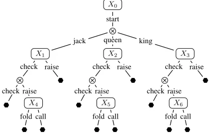
As an illustration, consider the game of Kuhn poker (Kuhn 1950). Kuhn poker consists of a three-card deck: king, queen, and jack. Each player is dealt one of the three cards and a single round of betting occurs. The action space for the first player is shown in Figure 1. For instance, we have:J =
{0,1,2,3,4,5,6};n0= 1, X0= ∆1={1};nj= 2, Xj= ∆2for allj ∈ J \ {0};A0 ={start},A1 =A2 = A3 = {check,raise},A4 = A5 = A6 = {fold,call}; C0,start =
{1,2,3},C1,raise = ∅, C3,check = {6};X41 = X1 ×X4, X44 =X4;x1= [x1,check, x1,raise];x41 = [x1;x4], etc.
In addition to games, our model captures, for example, POMDPs and MDPs where we condition on the entire history of observations and actions.
Sequence Form for Sequential Decision Processes
So far we have described the decision space as a product of convex sets where the choice of each action is taken from a subset of a simplexXj ⊆ ∆nj. This formulation has a
drawback: the expected-value function for a given strategy
X0
X3
X6
X2
X5
X1
X4
start
fold call fold call fold call
check raise check raise check raise
jack queen king
check raise check raise check raise
Figure 1: Sequential action space for the first player in the game of Kuhn poker. denotes an observation point; represents the end of the decision process.
is not linear. Consider taking actionaat decision pointj. In order to compute the expected overall contribution of that decision, its local payoffgj,ahas to be weighted by the prod-uct of probabilities of all actions on the path tojand byxj,a. So, the overall expected utility is nonlinear and non-convex. We now present a well-known alternative representation of this decision space which preserves linearity. While we will mainly be working in the product spaceX, it will occasion-ally be useful to move to this equivalent representation to preserve linearity.
The alternative formulation is called thesequence form.
In that representation, every convex setj ∈ J is scaled by the parent variable leading toj. In other words, the sum of values atj now sum to the value of the parent variable. In this formulation, the value of a particular action represents the probability of playing the whole sequenceof actions
from the root to that action. This allows each term in the expected loss to be weighted only by the sequence ending in the corresponding action. The sequence form has been used to instantiate linear programming (von Stengel 1996) and first-order methods (Hoda et al. 2010; Kroer et al. 2015; 2018) for computing Nash equilibria of zero-sum EFGs. There is a straightforward mapping between any x ∈ X to its corresponding sequence form: simply assign each sequence the product of probabilities in the sequence. Likewise, going from sequence form toXcan be done by dividing eachxj,a by the valuexpj wherepjis the entry inxcorresponding to
the parent ofj. We letµbe a function that maps eachx∈X to its corresponding sequence-form vector. For the reverse directionµ−1, there is ambiguity becauseµis not injective. Nonetheless, an inverse can be computed in linear time.
Regret in Sequential Decision Making
We assume that we are playing a sequence ofT iterations of a sequential decision process. At each iterationtwe choose a strategyx∈Xand are then given a loss function of the form`t(x) :=X j∈J
πj(x)`tj(xj), (1)
where`t
the product of the probability of each action in the path from the root of the tree to decision pointj. We coin loss functions of this formseparable, and they will play an important role
in our results. Our goal is to compute a new strategy vector xtsuch that the regret across allT iterations is as low as possible against any sequence of loss functions.
We now summarize definitions for the value and regret associated with convex sets and strategies. First we have the value of convex setjat iterationtwhen following strategyx:ˆ
ˆ
V4tj(ˆx4j) :=` t j(ˆxtj) +
X
a∈Aj X
j0∈Cj,a ˆ
xj,aVˆ4tj0(ˆx4j0). (2)
This definition denotes the utility associated with starting at convex set Xj rather than at the root. We will be par-ticularly interested in the value of xt, which we denote Vt
4j := ˆV
t 4j(x
t 4j).
Now we can define the cumulative regret at convex setj across allTiterations as
RT4j := T
X
t=1
V4tj −minxˆ
4j
T
X
t=1
ˆ
V4tj(ˆx4j),
This can equivalently be stated as
min
ˆ
x4j
T
X
t=1
ˆ
V4tj(ˆx4j) = T
X
t=1
V4tj−RT4j. (3)
Finally,average regretisR¯T 4j :=
1
TR T 4j.
Laminar Regret Decomposition
We now define a new parameterized class of loss functions for each subtreeXjwhich we will show can be used to minimize regret overXby minimizing that loss function independently at each convex setXj. The loss function is
ˆ
`tj:xj7→`tj(xj) +
X
a∈Aj X
j0∈Cj,a
xj,aV4tj0. (4)
It is convex since`t
j is convex by hypothesis and we are only adding a linear term to it. Strict convexity is also pre-served, and for strongly convex losses, the strong convexity parameter remains unchanged.
We now prove that the regret at information setj decom-poses into regret terms depending on`ˆt
jand a sum over the regret at child convex sets:
Theorem 1. The cumulative regret at a decision pointjcan be decomposed as
RT4j = T
X
t=1
ˆ
`tj(x t
)− min
ˆ
xj∈Xj
T
X
t=1
ˆ
`tj(ˆxj)−
X
a∈Aj X
j0∈C
j,a ˆ
xj,aRT4j0
Proof. By definition, the cumulative regretRT
4j at timeT
for decision pointjis:
T
X
t=1
V4tj−min
ˆ
x4j
T
X
t=1
`tj(ˆxj)+ T
X
t=1
X
a∈Aj X
j0∈C
j,a ˆ
xj,aVˆ4tj0(ˆx4j0)
= T
X
t=1
V4tj −ˆxmin j∈Xj
T
X
t=1
`tj(ˆxj)
+ X
a∈Aj X
j0∈Cj,a
ˆ
xj,amin
ˆ
x4j0
T
X
t=1
ˆ
V4tj0(ˆx4j0)
, (5)
where the equalities follow first from expanding the defini-tions ofRT
4j andVˆ
t
4j(ˆx4j), and then using the fact that we
can sequentially minimize first over choices atj and then over choices for child information sets.
Now we can use (3) to get that (5) is equal to
= T
X
t=1
V4tj− min
ˆ
xj∈Xj
T
X
t=1
ˆ
`tj(ˆxj)−
X
a∈Aj ˆ
xj,a
X
j0∈Cj,a Rt4j0
. (6)
SinceVt
4j already depends onV
t
4j0 for each child decision
pointj0we haveVt 4j = ˆ`
t j(x
t
j), where the equality follows by the definition of`ˆt
j. Substituting this equality in (6) yields the statement.
Theorem 1 justifies the introduction of the concept of lam-inar regretat each decision pointj ∈ J:
ˆ
RTj := T
X
t=1
ˆ
`tj(x t
j)− min
ˆ
xj∈Xj T
X
t=1
ˆ
`tj(ˆxj).
With this, we can write the cumulative subtree regret at decision pointj as a sum of laminar regret atj plus a re-currence term for each child decision point. Applying this inductively gives the following theorem which tells us how one can apply regret minimization locally on laminar regrets in order to minimize regret in SDMs:
Theorem 2. The cumulative regret onXsatisfies
RT ≤max
ˆ
x∈X
X
j∈J
πj(ˆx) ˆRTj.
Corollary 1. If each individual laminar regretRˆT
j on each
of the convex domainsXjgrows sublinearly, overall regret
onXgrows sublinearly.
Theorem 2 shows that overall regret can be minimized by minimizing each laminar regret separately. In particular, this means that if we have a regret minimizer for each decision pointjthat can handle the structure of the convex setXjand the convex loss from (4), then we can apply those regret min-imizers individually at each information set, and Theorem 2 guarantees that overall regret will be bounded by a weighted sum over those local regrets. For example, if each local regret minimizer has regret that grows at a particular sublinear rate, then the overall regret is also guaranteed to grow only at that sublinear rate.
Algorithm 1 gives pseudocode for a sample implemen-tation of a regret minimizer based on LRD. The algorithm assumes that a regret minimizerRjhas been chosen for each decision pointj ∈ J and has been initialized via a call to Rj.INITIALIZE()before the algorithm starts. A concrete ex-ample of regret local regret minimizerRj based on online gradient descent (OGD) is given later, together with its imple-mentation, in Algorithm 2. The algorithm first iterates over all actions and associated child information sets. For each child information setj0the subtree strategyxt
4j0is requested, then
the subtree valueVt
4j is computed, and finally it recurses by
observing loss atj0. By observing loss atj0after requesting xt
4j0 we ensure thatV
t
Algorithm 1Regret minimizer based on LRD 1: functionSDMOBSERVELOSS(j,{`t
k}k∈J)
2: fora∈Ajdo
3: forj0∈ Cj,ado
4: xt4j0 ←SDMRECOMMEND(j
0
)
5: Vt
4j ← Value of strategyx t
4j0 as defined in (2)
6: SDMOBSERVELOSS(j0,{`tk}k
∈J)
7: Construct`ˆjas defined in (4) using`j, the strategiesxt j0
and the valuesV4tjcomputed at lines 4 and 5 above.
8: Rj.OBSERVELOSS(ˆ`j)
1: functionSDMRECOMMEND(j)
2: xj← Rj.RECOMMEND()
3: fora∈Ajdo
4: forj0∈ Cj,ado
5: x4j0 ←SDMRECOMMEND(j
0
)
6: returnstrategyx4jdefined byxjatjandx4j0 for each
subtree4j0.
prior to observing the loss at roundt. Finally the local regret minimizerRjobserves the loss.
Our result gives an alternative proof of CFR. This is ar-guably simpler than existing proofs, because we show directly why regret over a sequential decision-making space decom-poses into individual regret terms, as opposed to bounding terms in order to fit the CFR framework. Finally, our result also generalizes CFR to new settings: we show how CFR can be implemented on arbitrary convex subsets of simplexes and with convex losses rather than linear.
Application Domains
Because we only need a finite sequential tree structure of the decision space, our framework captures a very broad class of SDM problems. In this section we describe how our frame-work can be applied to a number of prominent applications, such as POMDPs and EFGs. In general, our framework can be applied to any SDM problem where one or more agents are faced with a finite sequence of decisions that form a tree, such that agents always remember all past actions. The spe-cific decision problem at each stage may depend on the past decisions as well as stochasticity. The fact that we require the decision space to be tree structured might seem limiting from the perspective of compactly representing the decision space. However, this has successfully been dealt with in applications by using state- or value-estimation techniques, rather than fully representing the original problem (Moravˇc´ık et al. 2017; Jin, Levine, and Keutzer 2018).
One example class of a single-agent decision problems that we can model is finite-horizon POMDPs where the his-tory of states and actions is remembered. In that case, each decision point corresponds to a specific sequence of actions and observations made by the agent. This setting is reminis-cent of the POMDP setting considered by Jin, Levine, and Keutzer (2018). This type of model can be used to model sequential medical treatment planning when combined with results on imperfect-recall abstraction (Lanctot et al. 2012; Chen and Bowling 2012; Kroer and Sandholm 2016a), and
has potential applications in steering evolutionary adapta-tion (Sandholm 2015; Kroer and Sandholm 2016b). Our framework allows more general models for such problems via our generalization to convex decision points and convex losses; for example our framework could be used for regular-ized models. For instance in a medical settings, we may want to regularize the complexity of the treatment plan.
Extensive-Form Games with Convex-Concave
Saddle-Point Structure
In extensive-form game with perfect recall each player faces a sequential decision-making problem, of the type described in the previous section and in Figure 1. The set of next potential decision pointsCj,a is based on observations of stochastic outcomes and actions taken by the other players.
Here, we will focus on two-player zero-sum EFGs with perfect recall, but with slightly more general utility structure than is usually considered. In particular, we assume that we are solving a convex-concave saddle-point problem of the following form:
min x∈Xmaxy∈Y
µ(x)>Aµ(y) +d1(µ(x))−d2(µ(y)) , (7)
whereX is the SDM polytope for Player1andY is the SDM polytope of Player2. Eachdiis assumed to be a dilated convex function of the form
di(µ(x)) =
X
j∈J
µ(x)pjdj
µ(x)j
µ(x)pj
=X
j∈J
πj(x)`j(xj),
that is, in the form given in (1).
In standard zero-sum EFGs, the loss function for each player at each iterationtis defined to be the negative payoff vector associated with the sequence-form strategy of the other player at that iteration; since we additionally allow a regu-larizationterm we also get a nonlinear convex term. More
formally, at each iterationt, the loss functions`t
X:X →R
and`t
Y :Y →Rfor player 1 and 2 respectively are defined as
`tX :x7→ −µ(x)>Aµ(yt) +d1(x),
`t
Y :y7→ µ(xt)
>
Aµ(y) +d2(y),
whereAis the sequence-form payoff matrix of the game (von Stengel 1996). Some simple algebra shows that`t
Xand` t Y are indeed separable (that is, they can be written in the form of Equation 1), where each decision-point-level loss`t
j,Xand `t
j,Y is a convex function.
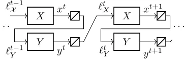
This choice of loss function is justified by the fact that the induced regret-minimizing dynamics for the two players lead to a convex-concave saddle-point problem. Specifically, assume the two players play the gameTtimes, accumulating regret after each iteration as in Figure 2.
A folk theorem explains the tight connection between low-regret strategies and approximate Nash equilibria. We will need a more general variant of that theorem generalized to (7). The convergence criterion we are interested in is the
saddle-point residual (or gap)ξof(¯x,y¯), defined as
ξ= max
ˆ
y {d1(¯x)−d2(ˆy)+ ¯x
>
Ayˆ} −min
ˆ
x {d1(ˆx)−d2(¯y)+ ˆx
> Ay¯}.
X
Y `tX−1
`tY−1
xt
yt `t Y `t
X X
Y xt+1
yt+1· · · · · ·
Figure 2: The flow of strategies and losses in regret min-imization for games. The symbol denotes computa-tion/construction of the loss function.
it has been stated in the form here. A closely related form is used for averaged strategy iterates in a first-order method by Nemirovski (2004).
Theorem 3. If the average regret accumulated onX and
Y by the two sets of strategies{xt}Tt=1 and{yt}Tt=1 is1
and2, respectively, then any strategy profile (¯x,y¯)such
thatµ(¯x) = 1
T PT
t=1µ(xt), µ(¯y) =T1 PT
t=1µ(yt)has a
saddle-point residual bounded by1+2.
The above averaging is performed in the sequence-form space, which works because that space is also convex. After averaging we can easily computex¯in linear time. Hence, by applying LRD to the decision spacesXandY, we converge to a small saddle-point residual. The fact that the averaging of the strategies is performed in sequence form explains why the traditional CFR presentation requires averaging with weights based on the player’s reachesπjat each decision pointj.
Theorem 3 shows that a Nash equilibrium can be com-puted by taking the uniform distribution over sequence-form strategy iterates. However, in the practical EFG-solving lit-erature another approach calledlinear averaginghas been
popular Tammelin et al. (2015), especially for the CFR+ al-gorithm. In linear averaging a weighted average strategy is constructed, where each strategyµ(xt)is weighted byt. Tam-melin et al. (2015) show that this is guaranteed to converge specifically when using the RM+regret minimizer. It would be interesting to prove when this works more generally. Here we make the simple observation that we can computeboth
averages, and simply use the one with better practical perfor-mance, even in settings where only the uniform average is guaranteed to converge.
Quantal Response Equilibrium (QRE) Ling, Fang, and
Kolter (2018) show that a reduced-normal-form logit QRE can be expressed as the convex-concave saddle-point prob-lem (7) where d1 and d2 are the (convex) dilated en-tropy functions usually used in first-order methods (FOMs) for solving EFGs (Hoda et al. 2010; Kroer et al. 2015; 2018). This saddle-point problem can be solved using FOMs, which would lead to fast convergence rate due to the strongly convex nature of the dilated entropy distance (Kroer et al. 2018). However, until now, no algorithms based on local re-gret minimization at each decision point have been known for this problem. Because the dilated entropy function sep-arates into a sum over negative entropy terms at each deci-sion point it can be incorporated as a convex loss in LRD. Combined with any regret-minimization algorithm that al-lows convex functions over the simplex, this leads to the first regret-minimization algorithm for computing (reduced-normal-form) logit QREs.
Perturbed EFGs and Equilibrium Refinement
Equilib-rium refinements are Nash equilibria with additional impor-tant rationality properties. Such equilibria have rarely been used in practice due to scalability issues. Recently, fast al-gorithms for computing approximate refinements were intro-duced (Kroer, Farina, and Sandholm 2017; Farina, Kroer, and Sandholm 2017). Theorem 1 gives a new tool for construct-ing such methods: it immediately implies correctness of the method of Farina, Kroer, and Sandholm (2017), while also allowing new types of refinements and regret minimizers.
Erratum about Alternation in CFR
+ Several tweaks to speed up the convergence of CFR have been proposed. The state of the art is CFR+(Tammelin et al. 2015). CFR+consists of three tweaks: the RM+ regret minimizer, linear averaging, and alternation. RM+ can be applied in our setting as well; it is simply an alternative regret minimizer for linear losses over a simplex. We described linear averaging earlier in this paper. Finally,alternationisthe idea that at iterationt, we provide Player2with the utility vector associated with thecurrentiterate of Player1, rather
than that of the previous iteration, as is normally done in regret minimization. Figure 3 illustrates how this works, in contrast with Figure 2 which shows the usual flow. Tammelin et al. (2015) state that they prove convergence of CFR+; however their proof relies on the folk theorem that links Nash equilibrium and regret. That folk theorem is only proven for the case where no alternation is applied. We show below that the theorem does not hold with alternation!
X
Y `t−1
X xt
yt `tY−1
`t X
X
Y xt+1
`t
Y yt+1
· · · · · ·
Figure 3: The alternation method for CFR in games. The loss at iterationtforyis computed withxt. The symbol denotes computation/construction of the loss function.
Observation 1. Let the action spaces for the players be
X =Y = [0,1], and let`t
X:x7→x·yt,`tY :y7→ −y·xt+1
be bilinear loss functions (the superscriptt+ 1comes from the use of alternation—see Figure 3). Consider the sequence of strategiesxt=t mod 2, yt= (t+ 1) mod 2. A simple
check reveals that after 2T iterations, the average regrets of the two players are both 0. Yet, the average strategies ¯
to an equilibrium at all. By our counterexample, if CFR+is sound, the proof will need to go through a different theorem than the folk theorem, and may need to leverage specific struc-ture of the regret minimizer, or may even need constraints on the initialization (for example, starting from the interior of the strategy space).
Experiments
We conducted experiments on two EFG settings. The first game is Leduc 5 poker (Southey et al. 2005), a standard benchmark in imperfect-information game solving. There is a deck consisting of 5 unique cards with 2 copies of each. There are two rounds. In the first round, each player places an ante of1in the pot and receives a single private card. A round
of betting then takes place with a two-bet maximum, with Player 1 going first. A public shared card is then dealt face up and another round of betting takes place. Again, Player 1 goes first, and there is a two-bet maximum. If one of the players has a pair with the public card, that player wins. Otherwise, the player with the higher card wins. All bets in the first round are1, while all bets in the second round are2.
The second game is a variant of Goofspiel (Ross 1971), a bidding game where each player has a hand of cards num-bered1toN. A third stack ofN cards is shuffled and used as prizes: each turn a prize card is revealed, and the players each choose a private card to bid on the prize, with the high card winning, the value of the prize card is split evenly on a tie. AfterN turns all prizes have been dealt out and the payoff to each player is the sum of prize cards that they win. We usedN= 4in our experiments.
We conducted three types of experiment, as described in the following subsections, respectively. Our code is parallel and the experiments were conducted on a machine with 8 cores, but the results are not about timing, so they would be identical even on a single core. We used alternation (Figure 3) only in the implementation of CFR+; all other algorithms use the flow of Figure 2.
Entropic Regularization Applied to Finding a
Quantal Response Equilibrium
First we investigated a setting where no previous regret-minimization algorithms based on minimizing regret locally existed: the computation of logit QREs via LRM and our more general convex losses. Ling, Fang, and Kolter (2018) used Newton’s method for this setting, but, as with Nash equilibrium, second-order algorithms do not scale to large games (this is why CFR+ has been so successful for cre-ating human-level poker AIs). We compared how quickly we could compute a logit QRE1compared to how quickly
a Nash equilibrium could be computed, in order to under-stand the size of games for which we can find a QRE with our approach. To do this, we ran LRM with online gradient descent (OGD) at each decision point. Because OGD is not guaranteed to stay within the simplex at each iteration, we needed to project onto the simplex. There are multiple fast
1For simplicity, we computed a logit QRE with parameterλ= 1.
However, our construction can easily be extended to handle any positive value ofλ.
ways of doing so, for example, a binary search (Duchi et al. 2008). The results are in Figure 4. LRM performs extremely well. In Goofspiel it converges vastly faster than CFR+, and in Leduc 5 it converges at a rate comparable to CFR+and eventually becomes faster. This shows that logit QRE compu-tation via LRM likely scales to extremely large EFGs, such as real-world-sized poker games (since CFR+is known to scale to such games).
101 102 103 104
10−6 10−4 10−2 100
Goofspiel 4 CFR+
Goofspiel
4
Leduc 5 CFR+
Leduc 5
Iteration
Saddle
point
gap
Quantal response equilibrium (entropic regularization)
Figure 4: The QRE saddle-point gap as a function of the number of iterations for each game. The convergence rates of CFR+for Nash equilibrium is shown for reference.
Quadratic Regularization: Using Strong Convexity
to Converge Faster
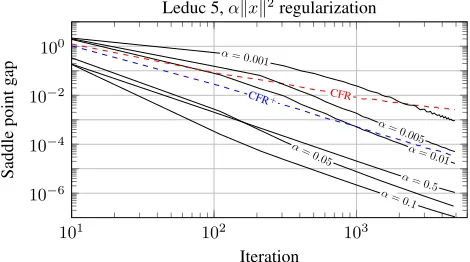
In the second set of experiments we investigated the speed of convergence for solving`2-regularized EFGs. In other words, at each decision point, we added to the loss a termαkzk2, wherezis the strategy at that decision point. Again we in-cluded the convergence rate of standard CFR and CFR+for Nash equilibrium computation as a benchmark. The results for Leduc 5 are in Figure 5. Solving the regularized game is significantly faster than computing a Nash equilibrium via CFR+, except for extremely small amounts of regularization.
101 102 103
10−6 10−4 10−2 100
α= 0 .01
CFR CFR+
α= 0 .5
α= 0 .1
α= 0 .05
α= 0 .005
α= 0.001
Iteration
Saddle
point
gap
Leduc 5,αkxk2regularization
The best speed is associated with an interior value ofα. This is because there is a tradeoff between stronger convex-ity (achieved by largerα) and smaller loss function values (achieved by smallerα). Algorithm 2 complements Algo-rithm 1 by providing pseudocode for the local regret mini-mizersRj that implement the quadratic regularization we just discussed.
Algorithm 2Local regret minimizers used in the quadratic
regularization experiments
1: functionRj.INITIALIZE( )
2: self.x←any strategy inXj= ∆nj (we used1/nj)
1: functionRj.OBSERVELOSS(`)
2: x˜←self.x− 1 2α√t∇`(x
t )
3: self.x←projectx˜ontoXj= ∆nj
1: functionRj.RECOMMEND( ) 2: returnself.x
Opponent Exploitation While Staying Close to a
Safe Strategy
In the third set of experiments we investigated the perfor-mance of LRM in a single-agent-learning setting: learning how to exploit a static opponent where we observe repeated samples from their strategy. We considered a setting where the exploiter wishes to maximally exploit subject to stay-ing near a pre-computed Nash equilibrium in order to avoid opening herself up to exploitability (Ganzfried and Sandholm 2011). We modeled this in a new way: as a regularized online SDM problem, where the loss for the exploiter is
`t:x
7→ −µ(x)>Aµ(yt) +αD(x
kxN E) (8) whereytis thet’th observation from the opponent’s strategy andD(xkxN E)is the dilated`
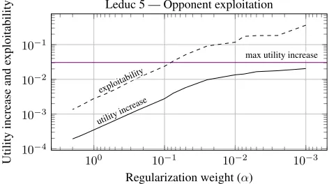
2-based Bregman divergence between the NE strategyxN Eandx. The opponent’s subop-timal strategy was computed by running CFR+until a gap of 0.1 was reached. We stopped the training of the exploiter after 5000 iterations or when an average regret of 0.0005 was reached, whichever happened first. Figure 6 shows the results. The “utility increase” line shows how much the agent gains by moving away from the Nash equilibrium and towards an exploitative strategy, while the “exploitability” shows to what extent the agent thereby opens herself up to being ex-ploited by her nemesis, that is, a best-response strategy of the opponent. We see that this model can indeed be used as a scalable proxy for trading off exploitation and exploitability by varyingα.
Conclusions and Future Research
We presented laminar regret decomposition (LRD), a new de-composition of the regret associated with a sequential action space into regrets associated with individual decision points. We developed our technique for general compact convex sets and convex losses at each decision point, thus providing a gen-eralization of CFR beyond simplex decision points and linear loss. We then showed that our results lead to a new class of regret-minimization algorithms that solve sequential decision
10−3 10−2
10−1 100
10−4 10−3 10−2 10−1
utilityincrease
max utility increase
exploitability
Regularization weight (α)
Utility
increase
and
exploitability
Leduc 5 — Opponent exploitation
Figure 6: The utility increase from exploitation, and the re-sulting increase in the agent’s exploitability, as a function of decreasing penalization on distance from Nash equilibrium in (8). The horizontal line shows the value of best responding to (that is, maximally exploiting) the opponent strategy.
making problems by minimizing regret locally at each deci-sion point. Although more general, our proof also provides a new perspective on the CFR algorithm in terms of our regret decomposition, and we explained the need for weighting by reach as a consequence of averaging in sequence form. We then showed that our approach can be used to compute reg-ularized equilibria as well as Nash equilibrium refinements, and gave the first regret-minimization algorithm for com-puting (reduced-normal-form) quantal response equilibrium (QRE) (based on local regrets). We showed experimentally that our framework, laminar regret minimization (LRM), can be used to compute QREs in extensive-form games (EFGs) at a rate that is comparable to Nash equilibrium finding using CFR+, thus yielding the first algorithm for computing QREs in large EFGs. We also showed that`2-regularized equilib-rium can be computed very quickly with out method. Finally, we showed how our approach can be used as a new approach to opponent exploitation, and to control the tradeoff between exploitation and exploitability.
de-composition so they can operate at the decision-point level, thereby having a better understanding of the problem struc-ture and allowing different algorithmic strategies to be used in different parts of the search space, etc.
Another opportunity presented by the strong convexity of the laminar losses is to use accelerated methods. This could lead to a faster theoretical convergence rate than that of CFR+for Nash equilibrium, and could likely be exploited in practice also. Furthermore, we used online gradient descent for convenience, but one could likely employ a projection-free algorithm and thus have the computational cost at each decision point be the same as for CFR+while having a faster convergence rate.
Another future direction is to extend the very recent im-provements to CFR and CFR+(Brown and Sandholm 2019), which were developed in parallel with this paper, to our set-ting. This may involve two directions: 1) generalizing those results to our more general settings, and 2) using those tech-niques to enhance the local regret minimizers at each decision point in our framework.
It would also be interesting to find further applications where our new types of decision spaces and loss functions can be used.
Acknowledgments
This material is based on work supported by the National Science Foundation under grants IIS-1718457, IIS-1617590, and CCF-1733556, and the ARO under award W911NF-17-1-0082. Christian Kroer was supported by a Facebook Fellowship.
References
Blackwell, D. 1956. An analog of the minmax theorem for vector payoffs.Pacific Journal of Mathematics.
Bowling, M.; Burch, N.; Johanson, M.; and Tammelin, O. 2015. Heads-up limit hold’em poker is solved.Science.
Brown, N., and Sandholm, T. 2017a. Safe and nested subgame solving for imperfect-information games. InNIPS.
Brown, N., and Sandholm, T. 2017b. Superhuman AI for heads-up no-limit poker: Libratus beats top professionals.Science.
Brown, N., and Sandholm, T. 2019. Solving imperfect-information games via discounted regret minimization. InAAAI.
Brown, N.; Kroer, C.; and Sandholm, T. 2017. Dynamic threshold-ing and prunthreshold-ing for regret minimization. InAAAI.
Chen, K., and Bowling, M. 2012. Tractable objectives for robust policy optimization. InNIPS.
Duchi, J.; Shalev-Shwartz, S.; Singer, Y.; and Chandra, T. 2008. Efficient projections onto the l1-ball for learning in high dimensions. InICML. ACM.
Farina, G., and Gatti, N. 2017. Extensive-form perfect equilibrium computation in two-player games. InAAAI.
Farina, G.; Kroer, C.; and Sandholm, T. 2017. Regret minimization in behaviorally-constrained zero-sum games. InICML.
Ganzfried, S., and Sandholm, T. 2011. Game theory-based opponent modeling in large imperfect-information games. InAAMAS.
Hart, S., and Mas-Colell, A. 2000. A simple adaptive procedure leading to correlated equilibrium.Econometrica.
Hazan, E., and Kale, S. 2010. Extracting certainty from uncertainty: Regret bounded by variation in costs. Machine learning.
Hazan, E. 2016. Introduction to online convex optimization. Foun-dations and Trends in Optimization.
Hoda, S.; Gilpin, A.; Pe˜na, J.; and Sandholm, T. 2010. Smooth-ing techniques for computSmooth-ing Nash equilibria of sequential games.
Mathematics of Operations Research.
Jin, P. H.; Levine, S.; and Keutzer, K. 2018. Regret minimization for partially observable deep reinforcement learning. InICML.
Kroer, C., and Sandholm, T. 2016a. Imperfect-recall abstractions with bounds in games. InEC.
Kroer, C., and Sandholm, T. 2016b. Sequential planning for steering immune system adaptation. InIJCAI.
Kroer, C.; Waugh, K.; Kılınc¸-Karzan, F.; and Sandholm, T. 2015. Faster first-order methods for extensive-form game solving. InEC.
Kroer, C.; Waugh, K.; Kılınc¸-Karzan, F.; and Sandholm, T. 2018. Faster algorithms for extensive-form game solving via improved smoothing functions.Mathematical Programming.
Kroer, C.; Farina, G.; and Sandholm, T. 2017. Smoothing method for approximate extensive-form perfect equilibrium. InIJCAI.
Kuhn, H. W. 1950. A simplified two-person poker. InContributions to the Theory of Games. Princeton University Press.
Lanctot, M.; Gibson, R.; Burch, N.; Zinkevich, M.; and Bowling, M. 2012. No-regret learning in extensive-form games with imperfect recall. InICML.
Ling, C. K.; Fang, F.; and Kolter, J. Z. 2018. What game are we playing? End-to-end learning in normal and extensive form games. InIJCAI.
Moravˇc´ık, M.; Schmid, M.; Burch, N.; Lis´y, V.; Morrill, D.; Bard, N.; Davis, T.; Waugh, K.; Johanson, M.; and Bowling, M. 2017. Deepstack: Expert-level artificial intelligence in heads-up no-limit poker.Science.
Nemirovski, A. 2004. Prox-method with rate of convergence O(1/t) for variational inequalities with Lipschitz continuous monotone operators and smooth convex-concave saddle point problems.SIAM Journal on Optimization.
Nesterov, Y. 2005. Excessive gap technique in nonsmooth convex minimization.SIAM Journal of Optimization.
Ross, S. M. 1971. Goofspiel–the game of pure strategy.Journal of Applied Probability.
Sandholm, T. 2015. Steering evolution strategically: Computational game theory and opponent exploitation for treatment planning, drug design, and synthetic biology. InAAAI. Senior Member Track.
Southey, F.; Bowling, M.; Larson, B.; Piccione, C.; Burch, N.; Billings, D.; and Rayner, C. 2005. Bayes’ bluff: Opponent mod-elling in poker. InUAI.
Tammelin, O.; Burch, N.; Johanson, M.; and Bowling, M. 2015. Solving heads-up limit Texas hold’em. InIJCAI.
von Stengel, B. 1996. Efficient computation of behavior strategies.
Games and Economic Behavior.
Zinkevich, M.; Bowling, M.; Johanson, M.; and Piccione, C. 2007. Regret minimization in games with incomplete information. In
NIPS.