On Geometric Alignment in Low Doubling Dimension

The Thirty-Third AAAI Conference on Artificial Intelligence (AAAI-19)

On Geometric Alignment in Low Doubling Dimension

Hu Ding

School of Computer Science and Technology School of Data Science

University of Science and Technology of China He Fei, China, 230026

[email protected]

Mingquan Ye

Department of Computer Science and Engineering Michigan State University

East Lansing, MI, USA, 48824 [email protected]

Abstract

In real-world, many problems can be formulated as the align-ment between two geometric patterns. Previously, a great amount of research focus on the alignment of 2D or 3D pat-terns, especially in the field of computer vision. Recently, the alignment of geometric patterns in high dimension finds sev-eral novel applications, and has attracted more and more at-tentions. However, the research is still rather limited in terms of algorithms. To the best of our knowledge, most existing ap-proaches for high dimensional alignment are just simple ex-tensions of their counterparts for 2D and 3D cases, and often suffer from the issues such as high complexities. In this pa-per, we propose an effective framework to compress the high dimensional geometric patterns and approximately preserve the alignment quality. As a consequence, existing alignment approach can be applied to the compressed geometric pat-terns and thus the time complexity is significantly reduced. Our idea is inspired by the observation that high dimensional data often has a low intrinsic dimension. We adopt the widely used notion “doubling dimension” to measure the extents of our compression and the resulting approximation. Finally, we test our method on both random and real datasets; the experi-mental results reveal that running the alignment algorithm on compressed patterns can achieve similar qualities, comparing with the results on the original patterns, but the running times (including the times cost for compression) are substantially lower.

1

Introduction

Given two geometric patterns, the problem of alignment is to find their appropriate spatial positions so as to minimize the difference between them. In general, a geometric pat-tern is represented by a set of (weighted) points in the space, and their difference is often measured by some objective function. In particular, geometric alignment finds many ap-plications in the field of computer vision, such as image retrieval, pattern recognition, fingerprint and facial shape alignment, etc (Cohen and Guibas 1999; Maltoni et al. 2009; Cao et al. 2014). For different applications, we may have different constraints for the alignment, e.g., we allow rigid transformations for fingerprint alignment. In addition, Earth Mover’s Distance (EMD) (Rubner, Tomasi, and Guibas

Copyright c⃝2019, Association for the Advancement of Artificial Intelligence (www.aaai.org). All rights reserved.

2000) has been widely adopted as the metric for measur-ing the difference of patterns in computer vision, where its major advantage over other measures is the robustness with respect to noise in practice. Besides the computer vision ap-plications in 2D or 3D, recent research shows that a number of high dimensional problems can be solved by geometric alignments. We briefly introduce several interesting exam-ples below.

(1) The research on natural language processing has re-vealed that different languages often share some similar structure at the word level (Youn et al. 2016); in particu-lar, the recent study on word semantics embedding has also shown the existence of structural isomorphism across lan-guages (Mikolov, Le, and Sutskever 2013), and further finds that EMD can serve as a good distance for languages or doc-uments (Zhang et al. 2017; Kusner et al. 2015). Therefore, (Zhang et al. 2017) proposed to learn the transformation be-tween different languages without any cross-lingual super-vision, and the problem is reduced to minimizing the EMD via finding the optimal geometric alignment in high dimen-sion. (2) A Protein-Protein Interaction (PPI) network is a graph representing the interactions among proteins. Given two PPI networks, finding their alignment is a fundamen-tal bioinformatics problem for understanding the correspon-dences between different species (Malod-Dognin, Ban, and Prˇzulj 2017). However, most existing approaches require to solve the NP-hard subgraph isomorphism problem and often suffer from high computational complexities. To resolve this issue, (Liu et al. 2017) recently applied the geometric em-bedding techniques to develop a new framework based on geometric alignment in Euclidean space.(3)Other applica-tions of high dimensional alignment include domain adap-tation and indoor localization. Domain adapadap-tation is an im-portant problem in machine learning, where the goal is to predict the annotations of a given unlabeled dataset by deter-mining the transformation (in the form of EMD) from a la-beled dataset (Pan and Yang 2010); as the rapid development of wireless technology, indoor localization becomes rather important for locating a person or device inside a building. Recent studies show that they both can be well formulated as geometric alignments in high dimension. We refer the reader to (Courty et al. 2017) and (Yang, Wu, and Liu 2012) for more details.

research on the algorithms is still rather limited and far from being satisfactory. Basically, we need to take into account of the high dimensionality and large number of points of the geometric patterns, simultaneously. In particular, as the de-veloping of data acquisition techniques, data sizes increase fast and designing efficient algorithms for high dimensional alignment will be important for some applications. For ex-ample, due to the rapid progress of high-throughput se-quencing technologies, biological data are growing expo-nentially (Yin et al. 2017). In fact, even for the 2D and 3D cases, solving the geometric alignment problem is quite challenging yet. For example, the well-known iterative clos-est point (ICP) method (Besl and McKay 1992) can only guarantee to obtain a local optimum. More previous works will be discussed in Section 1.2.

To the best of our knowledge, we are the first to consider developing efficient algorithmic framework for the geomet-ric alignment problem in large-scale and high dimension. Our idea is inspired by the observation that many real-world datasets often manifest low intrinsic dimensions (Belkin 2003). For example, human handwriting images can be well embedded to some low dimensional manifold though the Euclidean dimension can be very high (Tenenbaum, De Silva, and Langford 2000). Following this observa-tion, we consider to exploit the widely used noobserva-tion, “dou-bling dimension” (Krauthgamer and Lee 2004; Talwar 2004; Karger and Ruhl 2002; Har-Peled and Mendel 2006; Das-gupta and Sinha 2013), to deal with the geometric alignment problem. Doubling dimension is particularly suitable to de-pict the data having low intrinsic dimension. We prove that the given geometric patterns with low doubling dimensions can be substantially compressed so as to save a large amount of running time when computing the alignment. More im-portantly, our compression approach is an independent step, and hence can serve as the preprocessing for various align-ment methods.

The rest of the paper is organized as follows. We provide the definitions that are used throughout this paper in Sec-tion 1.1, and discuss some existing approaches and our main idea in Section 1.2. Then, we present our algorithm, anal-ysis, and the time complexity in detail in Section 2 and 3. Finally, we study the practical performance of our proposed algorithm in Section 4.

1.1

Preliminaries

Before introducing the formal definition of geometric align-ment, we need to define EMD and rigid transformation first. Definition 1 (Earth Mover’s Distance (EMD)). Let A =

{a1, a2,· · ·, an1}andB={b1, b2,· · ·, bn2}be two sets of

weighted points inRd with nonnegative weightsαi andβj

for eachai ∈Aandbj ∈Brespectively, andWAandWB

be their respective total weights. The earth mover’s distance betweenAandBisEMD(A, B) =

1 min{WA, WB}

min

F n1

∑

i=1

n2

∑

j=1

fij||ai−bj||2, (1)

where F = {fij} is a feasible flow from A to B, i.e.,

each fij ≥ 0,

∑n1

i=1fij ≤ βj,

∑n2

j=1fij ≤ αi, and

∑n1

i=1

∑n2

j=1fij= min{WA, WB}.

Intuitively, EMD can be viewed as the minimum trans-portation cost between A andB, where the weights of A

andB are the “supplies” and “demands” respectively, and the cost of each edge connecting a pair of points fromAtoB

is their “ground distance”. In general, the “ground distance” can be defined in various forms, and here we simply use the squared distance because it is widely adopted in practice.

Definition 2 (Rigid Transformation). Let P be a set of points inRd. A rigid transformationT onP is a

transfor-mation (i.e., rotation, translation, reflection, or their combi-nation) which preserves the pairwise distances of the points inP.

We consider rigid transformation for alignment, because it is very natural to interpret in real-world and has already been used by the aforementioned applications.

Definition 3 (Geometric Alignment). Given two weighted point setsAandBas described in Definition 1, the problem of geometric alignment betweenAandBunder rigid trans-formation is to determine a rigid transtrans-formationT forBso as to minimize the earth mover’s distanceEMD(A,T(B)).

As previously mentioned, we consider to use doubling di-mension to describe high didi-mensional data having low in-trinsic dimension. We denote a metric space by (X, dX)

wheredXis the distance function of the setX. For instance,

we can imagine thatXis a set of points in a low dimensional manifold and dX is simply Euclidean distance. For any

x∈X andr ≥0,Ball(x, r) ={p∈X | dX(x, p)≤r}

indicates the ball of radiusraroundx(note thatBall(x, r) is a subset ofX).

Definition 4(Doubling Dimension). The doubling dimen-sion of a metric space (X, dX) is the smallest number ρ,

such that for anyx∈ X andr≥0,Ball(x,2r)is always covered by the union of at most2ρ_{balls with radiusr.}

Doubling dimension describes the expansion rate of (X, dX); intuitively, we can imagine a set of points

uni-formly distributed inside aρ-dimensional hypercube, where its doubling dimension is O(ρ) but the Euclidean dimen-sion can be very high. For a more general case, a mani-fold in high dimensional Euclidean space may have a very low doubling dimension, as many examples studied in ma-chine learning (Belkin 2003). Unfortunately, as shown be-fore (Laakso 2002), such low doubling dimensional metrics cannot always be embedded to low dimensional Euclidean spaces with low distortion in terms of Euclidean distance. Therefore, we need to design the techniques being able to manipulate the data in high dimensional Euclidean space di-rectly.

1.2

Existing Results and Our Approach

If building a bipartite graph, where the two columns of ver-tices correspond to the points ofAandB respectively and each edge connecting (ai, bj)has the weight ||ai −bj||2,

algo-rithm (Ahuja, Magnanti, and Orlin 1993), a specialized ver-sion of the simplex algorithm. Since EMD is an instance of min-cost flow problem in Euclidean space and the geometric techniques (e.g., the geometric sparse spanner) are applica-ble, a number of faster algorithms have been proposed in the area of computational geometry (Agarwal et al. 2017; Cabello et al. 2008; Indyk 2007), however, most of them only work for low dimensional case. Several EMD algo-rithms with assumptions (or some modifications on the objective function of EMD) have been studied in practi-cal areas (Pele and Werman 2009; Ling and Okada 2007; Benamou et al. 2015).

Computing the geometric alignment ofAandB is more challenging, since we need to determine the rigid trans-formation and EMD flow simultaneously. Moreover, due to the flexibility of rigid transformations, we cannot apply the EMD embedding techniques (Indyk and Thaper 2003; Andoni et al. 2009) to relieve the challenges. For example, the embedding can only preserve the EMD betweenAand

B; however, since there are infinite number of possible rigid transformationsT forB(note that we do not knowT in ad-vance), it is difficult to also preserve the EMD between A

andT(B). In theory, (Cabello et al. 2008) presented a(2 +

ϵ)-approximation solution for the 2D case, and later (Klein and Veltkamp 2005) achieved anO(2d−1)-approximation in

Rd; (Ding and Xu 2017) proposed a PTAS for constant

di-mension. However, these theoretical algorithms cannot be efficiently implemented when the dimensionality is not con-stant. (Ding and Xu 2017) also mentioned that any constant factor approximation needs a time complexity at leastnΩ(d) based on some reasonable assumption in the theory of com-putational complexity, wheren= max{|A|,|B|}. That is, it is unlikely to obtain a(1 +ϵ)-approximation within a prac-tical running time, especially whennis very large.

In practice, (Cohen and Guibas 1999) proposed an alter-nating minimization approach for computing the geometric alignment of A andB. Several other approaches (Cornea et al. 2005; Todorovic and Ahuja 2008) based on graph matching are inappropriate to be extended for high dimen-sional alignment. In machine learning, a related topic is called “manifold alignment” (Ham, Lee, and Saul 2005; Wang, Krafft, and Mahadevan 2011); however, it usually has different settings and applications, and thus is out of the scope of this paper.

Because the approach of (Cohen and Guibas 1999) is closely related to our proposed algorithm, we introduce it with more details for the sake of completeness. Roughly speaking, their approach is similar to the Iterative Closest Point method (ICP) method (Besl and McKay 1992), where its each iteration alternatively updates the EMD flow and rigid transformation. Thus it converges to some local opti-mum eventually. To update the rigid transformation, we can apply Orthogonal Procrustes (OP) analysis (Sch¨onemann 1966). The original OP analysis is only for unweighted point sets, and hence we need some significant modification for our problem.

Suppose that the EMD flowF = {fij} is fixed and the

rigid transformation is waiting to update in the current stage.

We imagine two new sets of weighted points ˆ

A = {a11, a21,· · · , a

n2

1 ;a 1

2, a22,· · · , a

n2

2 ;

· · · ;a1_n

1, a

2

n1,· · · , a

n2

n1}; (2)

ˆ

B = {b1₁, b1₂,· · · , b1_n2;b2₁, b2₂,· · ·, b2_n2;

· · · ;bn1

1 , b

n1

2 ,· · · , b

n1

n2}, (3)

where each aj_i (resp., bi_j) has the weight fij and the same

spatial position ofai(resp.,bj). With a slight abuse of

nota-tions, we also useaj_i (resp.,bi

j) to denote the corresponding

d-dimensional column vector in the following description. First, we take a translation vector−→v such that the weighted mean points ofAˆandBˆ+−→v coincide with each other (this can be easily proved, due to the fact that the objective func-tion uses squared distance (Cohen and Guibas 1999)). Sec-ond, by OP analysis, we compute an orthogonal matrixR

for Bˆ +−→v to minimize its weighted L2

2 difference toAˆ. For this purpose, we generate twod×(n1n2)matricesMA

andMB, where each point ofAˆ(resp.,Bˆ+−→v) corresponds

to an individual column of MA (resp., MB); for example,

a point aj_i ∈ Aˆ (resp., bi

j +−→v ∈ Bˆ +−→v) corresponds

to a column√fija j i (resp.,

√

fij(bij+

− →_{v)) inM}

A (resp.,

MB). Let the SVD ofMA×MBT beUΣV

T_{, and the optimal}

orthogonal matrixRshould beU VT through OP analysis. Actually we do not need to really construct the large matri-cesMA andMB, since many of the columns are identical.

Instead, we can compute the multiplication MA×MBT in

O(n1n2d+ min{n1, n2} ·d2)time (see Lemma 3 in Ap-pendix). Therefore, the time complexity for obtaining the optimalRisO(n1n2d+ min{n1, n2} ·d2+d3).

Proposition 1. Each iteration of the approach of (Co-hen and Guibas 1999) takes Γ(n1, n2, d) + O(n1n2d+ min{n1, n2}·d2+d3)time, whereΓ(n1, n2, d)indicates the time complexity of the EMD algorithm it adopts. In practice, we usually assumen1, n2 = O(n)with somen ≥ d, and then the complexity can be simplified to beΓ(n, d)+O(n2_d). The bottleneck is that the algorithm needs to repeatedly compute the EMD and transformation, especially when n

anddare large (usuallyΓ(n, d) = Ω(n2_{d)). Based on the} property of low doubling dimension, we construct a pair of compressed point sets to replace the original AandB, and run the same algorithm on the compressed data instead. As a consequence, the running time is reduced significantly. Note that our compression step isindependent ofthe ap-proach (Cohen and Guibas 1999); actually, any alignment method with the same objective function in Definition 3 can benefit from our compression idea. Recently, (Nasser, Jubran, and Feldman 2015) proposed a core-set based com-pression approach to speed up the computation of align-ment. However, their method requires to know the corre-spondences between the point sets in advance and therefore it is not suitable to handle EMD; moreover, their compres-sion achieves the advantage only whendis small.

2

The Algorithm and Analysis

space,k-center clustering is to partitionPintokclusters and cover each cluster by an individual ball, such that the maxi-mum radius of the balls is minimized. (Gonzalez 1985) pre-sented an elegant2-approximation algorithm, where the ra-dius of each resulting ball (i.e., cluster) is at most two times the optimum. Initially, it selects an arbitrary point, sayc1, from the inputP and setsS ={c1}; then it iteratively se-lects a new point which has the largest distance toSamong the points of P and adds it to S, until |S| = k (the dis-tance between a pointqandSis defined asmin{||q−p|| |

p ∈ S}); supposeS = {c1,· · · , ck}, and thenP is

cov-ered by thek ballsBall(c1, r),· · ·, Ball(ck, r)withr ≤

min{||ci−cj|| | 1 ≤ i ̸=j ≤ k}. It is able to prove that

r is at most two times the optimal radius of the given in-stance. Using the property of doubling dimension, we have the following lemma.

Lemma 1. LetPbe a point set inRdwith the doubling

di-mensionρ ≪ d. The diameter of P is denoted by∆, i.e., ∆ = max{||p−q|| | p, q ∈P}. Given a small parameter

ϵ >0, if one runs thek-center clustering algorithm of Gon-zalez by settingk = (2_ϵ)ρ, the radius of each resulting ball is at mostϵ∆.

Proof. Let S be the set of k points by Gonzalez’s algo-rithm, and the resulting radius be r. We also define the aspect ratio of S as the ratio between the maximum and minimum pairwise distances in S. Then, it is easy to see that the aspect ratio of S is at most ∆/r. Now, we need the following Claim 1 from (Krauthgamer and Lee 2004; Talwar 2004). Actually, the claim can be obtained by recur-sively applying the definition of doubling dimension.

Claim 1. Let(X, dX)be a metric space with the doubling

dimensionρ, andY ⊂X. If the aspect ratio ofY is upper bounded by some positive valueα, then|Y| ≤2ρ⌈log2α⌉_.

ReplacingXandY byPandSrespectively in the above claim, we have

|S| ≤2ρ⌈log2∆/r⌉≤₂ρ(1+log2∆/r)_{. (4)}

Since|S|= (2/ϵ)ρ_{, (4) impliesr≤ϵ∆.}

LetAandB be the two given point sets in Definition 3, and the maximum of their diameters be∆. We also assume that they both have the doubling dimension at mostρ. Our idea for compressingAandBis as follows. As described in Lemma 1, we setk = (2_ϵ)ρ and run Gonzalez’s algorithm onAandBrespectively. We denote bySA={cA1,· · ·, cAk}

andSB ={cB1,· · ·, cBk}the obtained sets ofk-cluster

cen-ters. For each cluster center cA_j (resp., cB_j), we assign a weight that is equal to the total weights of the points in the corresponding cluster. As a consequence, we obtain a new instance(SA, SB)for geometric alignment. It is easy

to know that the total weights ofSA (resp.,SB) is equal to

WA(resp.,WB). The following theorem shows that we can

achieve an approximate solution for the instance(A, B)by solving the alignment of(SA, SB).

Theorem 1. Suppose ϵ > 0 is a small param-eter in Lemma 1. Given any c ≥ 1, let T˜ be

a rigid transformation yielding c-approximation for minimizing EMD(

SA,T(SB)) in Definition 3. Then,

EMD(

A,T˜(B))

≤ c(1 + 2ϵ)2·min

T EMD

(

A,T(B))

+2ϵ(c+ 1 + 2cϵ)(1 + 2ϵ)∆2

= c(

1 +O(ϵ))

·min

T EMD

(

A,T(B))

+2ϵ(

1 +O(ϵ))

(c+ 1)∆2. (5)

Proof. First, we denote byToptthe optimal rigid

transfor-mation achieving minT EMD(A,T(B)). Since T˜ yields

c-approximation for minimizing EMD(

SA,T(SB) )

, we haveEMD(

SA,T˜(SB) )

≤ c·min

T EMD

(

SA,T(SB) )

≤ c· EMD(

SA,Topt(SB) )

. (6)

Recall that each point cA_j (resp., cB_j) has the weight equal to the total weights of the points in the cor-responding cluster. For instance, if the cluster contains

{aj(1), aj(2),· · ·, aj(h)}, the weight of cAj should be ∑h

l=1αj(l); actually, we can view cAj as h overlapping

points {a′_j(1), a′_j(2),· · · , a′_j(h)} with each a′_j(l) having the weightαj(l). Therefore, for the sake of convenience, we use another representation forSAandSBin our proof below:

SA={a′1,· · · , a′n1}andSB={b

′

1,· · · , b′n2}, (7)

where eacha′

j(resp.,b′j) has the weightαj(resp.,βj). Note

thatSAandSB only havekdistinct positions respectively

in the space. Moreover, due to Lemma 1, we know that

||a′_i −ai||, ||b′j −bj|| ≤ ϵ∆ for any 1 ≤ i ≤ n1 and 1≤j≤n2, and these bounds are invariant under any rigid transformation in the space. Consequently, for any pair(i, j) and rigid transformationT, we have||ai− T(bj)||2

≤ (

||ai−a′i||+||a′i− T(b′j)||

+||T(b′j)− T(bj)|| )2

≤ (

||a′_i− T(b′_j)||+ 2ϵ∆)2

= ||a′_i− T(b_j′)||2_{+ 4ϵ∆||a}′

i− T(b

′

j)||+ 4ϵ

2_∆2

≤ ||a′_i− T(b′_j)||2+ 2ϵ(

∆2+||a′_i− T(b′_j)||2)

+4ϵ2∆2

= (1 + 2ϵ)||a′_i− T(b_j′)||2_{+ (2ϵ+ 4ϵ}2_)∆2 ₍₈₎

by applying triangle inequality. Using exactly the same idea, we have||a′_i− T(b′_j)||2

≤(1 + 2ϵ)||ai− T(bj)||2+ (2ϵ+ 4ϵ2)∆2. (9)

Based on Definition 1, we denote by F˜ = {f˜ij} the

in-duced flow of EMD(

SA,T˜(SB) )

EMD(

A,T˜(B))

≤ 1

min{WA, WB} n1

∑

i=1

n2

∑

j=1 ˜

fij||ai−T˜(bj)||2

≤ 1 + 2ϵ

min{WA, WB} n1

∑

i=1

n2

∑

j=1 ˜

fij||a′i−T˜(b′j)||

2

+(2ϵ+ 4ϵ2)∆2

= (1 + 2ϵ)EMD(SA,T˜(SB))

+(2ϵ+ 4ϵ2)∆2. (10)

By the similar idea (replacing T˜ byTopt, and exchanging

the roles of(A, B)and(SA, SB)), (9) directly implies that

EMD(

SA,Topt(SB))

≤ (1 + 2ϵ)EMD(

A,Topt(B) )

+(2ϵ+ 4ϵ2)∆2. (11)

Combining (6), (10), and (11), we haveEMD(

A,T˜(B))

≤ (1 + 2ϵ)EMD(

SA,T˜(SB) )

+(2ϵ+ 4ϵ2)∆2

≤ (1 + 2ϵ)·c· EMD(

SA,Topt(SB) )

+(2ϵ+ 4ϵ2)∆2

≤ c(1 + 2ϵ)2· EMD(

A,Topt(B) )

+2ϵ(c+ 1 + 2cϵ)(1 + 2ϵ)∆2, (12)

and the proof is completed.

When ϵ is small enough, Theorem 1 shows that

EMD(

A,T˜(B))

≈ c· EMD(

A,Topt(B) )

. That is, T˜, the solution of(SA, SB), achieves roughly the same

perfor-mance on(A, B). Consequently, we propose the approxima-tion algorithm for geometric alignment (see Algorithm 1). We would like to emphasize that though we use the algo-rithm from (Cohen and Guibas 1999) in Step 3, Theorem 1 is an independent result; that is, any alignment method with the same objective function in Definition 3 can benefit from Theorem 1.

Algorithm 1Geometric Alignment 1: Givenϵ∈(0,1)and setk= (2/ϵ)ρ.

2: Run Gonzalez’sk-center clustering algorithm onAand

B, and obtain the sets of cluster centersSAandSB

re-spectively.

3: Apply the existing alignment algorithm, e.g., (Cohen and Guibas 1999), on(SA, SB).

4: Obtain the rigid transformation T from Step 3, and compute the corresponding EMD flow betweenAand

T(B).

5: Output: A rigid transformationT of B and the EMD flow betweenAandT(B).

3

The Time Complexity

We analyze the time complexity of Algorithm 1 and consider step 2-4 separately. To simplify our description, we usento denotemax{n1, n2}. In step 3, we suppose that the iterative approach (Cohen and Guibas 1999) takesλ≥1rounds.

Step 2.A straightforward implementation of Gonzalez’s algorithm is selecting thekcluster centers iteratively where the resulting running time isO(knd). Several faster imple-mentations for the high dimensional case with low doubling dimension have been studied before; their idea is to maintain some data structures to reduce the amortized complexity of each iteration. We refer the reader to (Har-Peled and Mendel 2006) for more details.

Step 3.Since we run the algorithm (Cohen and Guibas 1999) on the smaller instance(SA, SB)instead of(A, B),

we know that the complexity of Step 3 is O(λ(

Γ(k, d) +

k2_d+kd2_+d3))

by Proposition 1.

Step 4.We need to compute the transformedT(B)first and thenEMD(A,T(B)). Note that the transformationT is not off-the-shelf, because it is the combination of a sequence of rigid transformations from the iterative approach (Co-hen and Guibas 1999) in Step 3. Since it takes λ rounds,

T should be the multiplication ofλrigid transformations. We use(Rl,−→vl)to denote the orthogonal matrix and

trans-lation vector obtained in thel-th round for1 ≤ l ≤λ. We can updateBround by round: starting froml= 1, updateB

to beRlB+−→vlin each round; the whole time complexity

will beO(λnd2_{). In fact, we have a more efficient way by} computingT first before transformingB.

Lemma 2. Let(R,−→v)be the orthogonal matrix and trans-lation vector ofT. Then

R = Πλ_l=1Rl,

−

→_{v = (Π}λ

l=2Rl)−→v1+ (Πλl=3Rl)−→v2+

· · ·+Rλ−→vλ−1+−→vλ, (13)

andT(B)can be obtained inO(λd3+nd2)time.

Proof. The equations (13) can be easily verified by sim-ple calculations. In addition, we can recursively compute the multiplicationsΠλ

l=iRlfori=λ, λ−1,· · · ,1.

Conse-quently, the orthogonal matrixRand translation vector−→v

can be obtained inO(λd3_{)time. In addition, the complexity} for computingT(B) =RB+−→v isO(nd2_).

Lemma 2 provides a complexity significantly lower than the previous O(λnd2_{) (usually n is much larger than} d in practice). After obtaining T(B), we can compute

EMD(A,T(B))inΓ(n, d)time.Notethat the complexity Γ(n, d)usually isΩ(n2d), which dominates the complex-ity of Step 2 and the second termnd2_{in the complexity by} Lemma 2. As a consequence, we have the following theorem for the running time.

Theorem 2. Supposen= max{n1, n2} ≥dand the algo-rithm of (Cohen and Guibas 1999) takesλ≥1rounds. The running time of Algorithm 1 isO(λ(

Γ(k, d) +k2_d+kd2₊

d3))

Table 1: Random dataset: EMDs and running times of different compression levels.

γ 1/50 1/40 1/30 1/20 1/10 1 EMD 0.948 0.946 0.945 0.943 0.941 0.933 Time (s) 48.7 54.2 61.0 80.6 144.6 1418.2

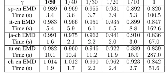
Table 2: Linguistic datasets: EMDs and running times of different compression levels.

γ 1/50 1/40 1/30 1/20 1/10 1 sp-en EMD 0.989 0.969 0.955 0.931 0.892 0.820

Time (s) 3.4 3.6 3.7 3.9 5.3 100.5 it-en EMD 0.983 0.966 0.951 0.935 0.899 0.847 Time (s) 5.4 5.9 6.1 6.5 8.8 162.6 ja-ch EMD 0.991 0.975 0.962 0.941 0.910 0.836 Time (s) 1.6 2.1 2.2 2.0 3.0 67.0 tu-en EMD 0.982 0.960 0.946 0.922 0.889 0.839

Time (s) 10.1 10.4 11.2 11.9 15.9 287.0 ch-en EMD 1.014 1.012 0.990 0.962 0.923 0.842 Time (s) 1.9 1.7 2.2 2.4 2.7 51.6

If we run the same number of rounds on the original in-stance(A, B)by the approach (Cohen and Guibas 1999), the

total running time will beO(λ(Γ(n, d) +n2d))by

Propo-sition 1. Whenk ≪ n, Algorithm 1 achieves a significant reduction on the running time.

4

Experiments

We implement our proposed algorithm and test the perfor-mance on both random and real datasets. All of the experi-mental results are obtained on a Windows workstation with 2.4GHz Intel Xeon CPU and 32GB DDR4 Memory. For each dataset, we run20trials and report the average results. We set the iterative approach (Cohen and Guibas 1999) to terminate when the change of the objective value is less than 10−3_.

To construct a random dataset, we randomly generate two manifolds inR500, which are represented by the polynomial

functions with low dimension (≤50); in the manifolds, we take two sets of randomly sampled points having the sizes ofn1 = 2×104 andn2 = 3×104, respectively; also, for each sampled point, we randomly assign a positive weight; finally, we obtain two weighted point sets as an instance of geometric alignment.

For real datasets, we consider the two applications men-tioned in Section 1, unsupervised bilingual lexicon induc-tion and PPI network alignment. For the first applicainduc-tion, we have 5 pairs of languages: Chinese-English, Spanish-English, Italian-Spanish-English, Japanese-Chinese, and Turkish-English. Given by (Zhang et al. 2017), each language has a vocabulary list containing3000to13000words; we also follow their preprocessing idea to represent all the words by vectors inR50 through the embedding technique (Mikolov,

Le, and Sutskever 2013). Actually, each vocabulary list is represented by a distribution in the space where each vec-tor has the weight equal to the corresponding frequency in the language. For the second application, we use the popu-lar benchmark dataset NAPAbench (Sayed Mohammad and

Yoon 2012) of PPI networks. It contains3pairs of PPI net-works, where each network is a graph of3000-10000nodes. As the step of preprocessing, we apply the recent node2vec technique (Grover and Leskovec 2016) to represent each network by a group of vectors in R100; following (Liu et

al. 2017), we assign a unit weight to each vector.

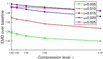
Results.For each instance, we try different compression levels. According to Algorithm 1, we compress the size of each point set to be k. We set k = γ×max{n1, n2} whereγ∈ {1/50,1/40,1/30,1/20,1/10,1}; in particular,

γ = 1indicates that we directly run the algorithm (Cohen and Guibas 1999) without compression. The purpose of our proposed approach is to design a compression method, such that the resulting qualities on the original and compressed datasets are close (as stated in Section 1.2 and the paragraph after the proof of Theorem 1). So in the experiment, we fo-cus on the comparison with the results on the original data (i.e., the results ofγ= 1).

The results on random dataset are shown in Table 1. The obtained EMDs by compression are only slightly higher than the ones ofγ= 1, while the advantage of the compression on running time is significant. For example, the running time ofγ= 1/50is less than5%of the one ofγ= 1. We obtain the similar performances on the real datasets. The results on Linguistic are shown in Table 2 (due to the space limit, we put the results on PPI network dataset in the full version of our paper); the EMD for each compression level is always at most1.2times the baseline withγ= 1, but the correspond-ing runncorrespond-ing time is dramatically reduced.

To further show the robustness of our method, we particu-larly add Gaussian noise to the random dataset and study the change of the objective value by varying the noise level. We set the standard variance of the Gaussian noise to beη×∆, where∆is the maximum diameter of the point sets andη

1/50 1/40 1/30 1/20 1/10 Compression level

1 1.02 1.04 1.06 1.08 1.1

EMD over baseline

=0.005 =0.010 =0.015 =0.020 =0.025

Figure 1: The EMDs over baseline for different noise levels.

5

Conclusion

In this paper, we propose a novel framework for compress-ing point sets in high dimension, so as to approximately pre-serve the quality of alignment. This work is motivated by several emerging applications in the fields of machine learn-ing, bioinformatics, and wireless network. Our method uti-lizes the property of low doubling dimension, and yields a significant speedup on alignment. In the experiments on ran-dom and real datasets, we show that the proposed compres-sion approach can efficiently reduce the running time to a great extent.

6

Acknowledgments

The research of this work was supported in part by NSF through grant CCF-1656905 and a start-up fund from Michi-gan State University. The authors also want to thank the anonymous reviewers for their helpful comments and sug-gestions for improving the paper.

7

Appendix

Lemma 3. The multiplicationMA×MBT can be computed

inO(n1n2d+ min{n1, n2} ·d2)time.

Proof. With a slight abuse of notations, we also useF to denote the n1 ×n2 matrix of the EMD flow where each entry isfij; also,Fi,: represents thei-th row of the matrix F. Given a vectort, we use√tto denote the new vector with each entry being the square root of the corresponding one in

t. Also, we usediag(t)to denote the diagonal matrix where thei-th diagonal entry is thei-th entry oft. Following the constructions ofMAandMB, we have

MA = [ √

f11a11,· · · ,

√

f1n2a

n2

1 ;

· · · ·

√

fn11a

1

n1,· · ·,

√

fn1n2a

n2

n1]

= [a1

√

F1,:, a2

√

F2,:,· · ·, an1

√

Fn1,:];

MB = [ √

f11b11,· · ·,

√

f1n2b

1

n2;

· · · ·

√

fn11b

n1

1 ,· · · ,

√

fn1n2b

n1

n2]

= B[diag(√F1,:),diag(

√

F2,:),

· · ·,diag(√Fn1,:)],

by some simple calculation. Then,

MA×MBT = n1

∑

i=1

(

ai √

Fi,:

)

×(

diag(√Fi,:)BT

)

=

n1

∑

i=1

aiFi,:BT =AF BT.

It is easy to know that computingAF BT _takesO(n

1n2d+ min{n1, n2} ·d2)time.

References

Agarwal, P. K.; Fox, K.; Panigrahi, D.; Varadarajan, K. R.; and Xiao, A. 2017. Faster algorithms for the geometric transportation problem. In 33rd International Symposium on Computational Geometry, SoCG 2017, July 4-7, 2017, Brisbane, Australia, 7:1–7:16.

Ahuja, R. K.; Magnanti, T. L.; and Orlin, J. B. 1993. Net-work flows: theory, algorithms, and applications. Prentice Hall.

Andoni, A.; Do Ba, K.; Indyk, P.; and Woodruff, D. 2009. Efficient sketches for earth-mover distance, with applica-tions. InFoundations of Computer Science, 2009. FOCS’09. 50th Annual IEEE Symposium on, 324–330. IEEE.

Belkin, M. 2003. Problems of learning on manifolds. The University of Chicago.

Benamou, J.; Carlier, G.; Cuturi, M.; Nenna, L.; and Peyr´e, G. 2015. Iterative bregman projections for regularized trans-portation problems. SIAM J. Scientific Computing37(2). Besl, P., and McKay, N. D. 1992. A method for registration of 3-d shapes. IEEE Transactions on Pattern Analysis and Machine Intelligence14(2):239–256.

Cabello, S.; Giannopoulos, P.; Knauer, C.; and Rote, G. 2008. Matching point sets with respect to the earth mover’s distance.Computational Geometry39(2):118–133.

Cao, X.; Wei, Y.; Wen, F.; and Sun, J. 2014. Face align-ment by explicit shape regression. International Journal of Computer Vision107(2):177–190.

Cohen, S., and Guibas, L. 1999. The earth mover’s distance under transformation sets. InProceedings of the 7th IEEE International Conference on Computer Vision, 1.

Cornea, N. D.; Demirci, M. F.; Silver, D.; Dickinson, S.; and Kantor, P. 2005. 3d object retrieval using many-to-many matching of curve skeletons. InShape Modeling and Appli-cations, 2005 International Conference, 366–371. IEEE.

Courty, N.; Flamary, R.; Habrard, A.; and Rakotomamonjy, A. 2017. Joint distribution optimal transportation for do-main adaptation. InAdvances in Neural Information Pro-cessing Systems, 3733–3742.

Dasgupta, S., and Sinha, K. 2013. Randomized partition trees for exact nearest neighbor search. InConference on Learning Theory, 317–337.

Gonzalez, T. F. 1985. Clustering to minimize the maximum intercluster distance.Theoretical Computer Science38:293– 306.

Grover, A., and Leskovec, J. 2016. node2vec: Scalable fea-ture learning for networks. InProceedings of the 22nd ACM SIGKDD International Conference on Knowledge Discov-ery and Data Mining, 855–864. ACM.

Ham, J.; Lee, D. D.; and Saul, L. K. 2005. Semisupervised alignment of manifolds. InAISTATS, 120–127.

Har-Peled, S., and Mendel, M. 2006. Fast construction of nets in low-dimensional metrics and their applications. SIAM Journal on Computing35(5):1148–1184.

Indyk, P., and Thaper, N. 2003. Fast color image retrieval via embeddings. InWorkshop on Statistical and Computational Theories of Vision (at ICCV).

Indyk, P. 2007. A near linear time constant factor approx-imation for euclidean bichromatic matching (cost). In Pro-ceedings of the eighteenth annual ACM-SIAM symposium on Discrete algorithms, 39–42. Society for Industrial and Applied Mathematics.

Karger, D. R., and Ruhl, M. 2002. Finding nearest neigh-bors in growth-restricted metrics. In Proceedings of the thiry-fourth annual ACM symposium on Theory of comput-ing, 741–750. ACM.

Klein, O., and Veltkamp, R. C. 2005. Approximation algo-rithms for computing the earth mover’s distance under trans-formations. InInternational Symposium on Algorithms and Computation, 1019–1028. Springer.

Krauthgamer, R., and Lee, J. R. 2004. Navigating nets: sim-ple algorithms for proximity search. InProceedings of the fifteenth annual ACM-SIAM symposium on Discrete algo-rithms, 798–807. Society for Industrial and Applied Mathe-matics.

Kusner, M.; Sun, Y.; Kolkin, N.; and Weinberger, K. 2015. From word embeddings to document distances. In Interna-tional Conference on Machine Learning, 957–966.

Laakso, T. J. 2002. Plane with a∞-weighted metric not

bilipschitz embeddable torn_{. Bulletin of the London}

Math-ematical Society34(6):667–676.

Ling, H., and Okada, K. 2007. An efficient earth mover’s distance algorithm for robust histogram comparison. IEEE transactions on pattern analysis and machine intelligence 29(5):840–853.

Liu, Y.; Ding, H.; Chen, D.; and Xu, J. 2017. Novel geo-metric approach for global alignment of PPI networks. In Proceedings of the Thirty-First AAAI Conference on Artifi-cial Intelligence, February 4-9, 2017, San Francisco, Cali-fornia, USA., 31–37.

Malod-Dognin, N.; Ban, K.; and Prˇzulj, N. 2017. Unified alignment of protein-protein interaction networks.Scientific Reports7(1):953.

Maltoni, D.; Maio, D.; Jain, A. K.; and Prabhakar, S. 2009. Handbook of fingerprint recognition. Springer Science & Business Media.

Mikolov, T.; Le, Q. V.; and Sutskever, I. 2013. Exploiting

similarities among languages for machine translation.arXiv preprint arXiv:1309.4168.

Nasser, S.; Jubran, I.; and Feldman, D. 2015. Low-cost and faster tracking systems using core-sets for pose-estimation. CoRRabs/1511.09120.

Pan, S. J., and Yang, Q. 2010. A survey on transfer learn-ing.IEEE Transactions on knowledge and data engineering 22(10):1345–1359.

Pele, O., and Werman, M. 2009. Fast and robust earth mover’s distances. InComputer vision, 2009 IEEE 12th in-ternational conference on, 460–467. IEEE.

Rubner, Y.; Tomasi, C.; and Guibas, L. J. 2000. The earth mover’s distance as a metric for image retrieval. Interna-tional journal of computer vision40(2):99–121.

Sayed Mohammad, E. S., and Yoon, B.-J. 2012. A network synthesis model for generating protein interaction network families.PloS one7.

Sch¨onemann, P. H. 1966. A generalized solution of the orthogonal procrustes problem. Psychometrika31(1):1–10. Talwar, K. 2004. Bypassing the embedding: algorithms for low dimensional metrics. InProceedings of the thirty-sixth annual ACM symposium on Theory of computing, 281–290. Tenenbaum, J. B.; De Silva, V.; and Langford, J. C. 2000. A global geometric framework for nonlinear dimensionality reduction. science290(5500):2319–2323.

Todorovic, S., and Ahuja, N. 2008. Region-based hierar-chical image matching. International Journal of Computer Vision78(1):47–66.

Wang, C.; Krafft, P.; and Mahadevan, S. 2011. Manifold alignment.

Yang, Z.; Wu, C.; and Liu, Y. 2012. Locating in fingerprint space: wireless indoor localization with little human inter-vention. In Proceedings of the 18th annual international conference on Mobile computing and networking, 269–280. ACM.

Yin, Z.; Lan, H.; Tan, G.; Lu, M.; Vasilakos, A. V.; and Liu, W. 2017. Computing platforms for big biological data analytics: perspectives and challenges. Computational and structural biotechnology journal15:403–411.