DEMOGRAPHIC RESEARCH
A peer-reviewed, open-access journal of population sciences
DEMOGRAPHIC RESEARCH
VOLUME 41, ARTICLE 38, PAGES 1091–1130
PUBLISHED 24 OCTOBER 2019
http://www.demographic-research.org/Volumes/Vol41/38/ DOI: 10.4054/DemRes.2019.41.38
Research Article
Smooth constrained mortality forecasting
Carlo G. Camarda
c
2019 Carlo G. Camarda.
This open-access work is published under the terms of the Creative Commons Attribution 3.0 Germany (CC BY 3.0 DE), which permits use, reproduction, and distribution in any medium, provided the original author(s) and source are given credit.
1 Introduction 1092
2 P-splines for mortality data 1095
2.1 Forecasting withP-splines 1099
3 TheCP-spline model 1102
3.1 Addressing infant mortality 1102
3.2 Enforcing mortality patterns over age and time 1104
3.2.1 Incorporating prior knowledge into the model 1110
3.2.2 Confidence intervals by bootstrap 1111
4 Application 1113
5 Conclusions 1118
6 Acknowledgments 1121
Smooth constrained mortality forecasting
Carlo G. Camarda1
Abstract
BACKGROUND
Mortality can be forecast by means of parametric models, principal component methods, and smoothing approaches. These methods either impose rigid modeling structures or produce implausible outcomes.
OBJECTIVE
We propose a novel approach for forecasting mortality that combines a well established smoothing model and prior demographic information. We constrain future smooth mor-tality patterns to lie within a range of valid age profiles and time trends, both computed from observed patterns.
METHODS
Within aP-spline framework, we enforce shape constraints through an asymmetric penalty approach on forecast mortality. Moreover, we properly integrate infant mortality in a smoothing framework so that the mortality forecast covers the whole age range.
RESULTS
The proposed model outperforms the plain smoothing approach as well as commonly used methodologies while retaining all the desirable properties that demographers expect from a forecasting method, e.g., smooth and plausible age profiles and time trends. We illustrate the proposed approach to mortality data for Danish females and US males.
CONCLUSIONS
The proposed methodology offers a new paradigm in forecasting mortality, and it is an ideal balance between pure statistical methodology and traditional demographic models. Prior knowledge about mortality development can be conveniently included in the ap-proach, leading to large flexibility. The combination of powerful statistical methodology and prior demographic information makes the proposed model suitable for forecasting mortality in most demographic scenarios.
1. Introduction
Mortality modeling and forecasting are crucial in epidemiology and population studies, as well as in the insurance and pensions industries. In recent decades, several methodologies have been proposed, and many demographers, actuaries, and statisticians have suggested approaches for projecting mortality. (See Booth and Tickle (2008) and Cairns, Blake, and Dowd (2008) and the references therein.)
In addition to scenario- and expert-based approaches in this growing body of meth-ods, we can broadly distinguish three classes based on their assumptions. A traditional procedure relies on using parametric models to describe mortality age patterns and then extrapolating the estimated parameters to reconstruct future mortality (see, among others, Tabeau, Willekens, and van Poppel (2002)). When dealing with adult mortality, para-metric models are extremely parsimonious, but a large number of parameters are often necessary when the whole age range is considered. Although these models present the advantage of a clear-cut interpretation of their parameters, this feature is not particularly useful in a forecasting approach. Moreover, when dealing with the whole age range, it is generally hard to disentangle the meaning attached to each parameter and simultaneously forecast plausible mortality patterns based on their time series.
Overparametrized models such as that of Lee and Carter (1992) and its variants have been widely used and have become a benchmark for many newly proposed method-ologies. They describe mortality development over age and time using their principal components. They reduce a two-dimensional problem to a fixed-age effect with a uni-variate time index. The time index condenses the mortality changes in past years and is thus used to forecast future mortality. This class of models presents several drawbacks, however. A simple univariate time series results in mortality improvements at all ages being perfectly correlated. Due to a fixed-age effect over time, lack of smoothness in the estimated mortality pattern is evident, especially in the forecast years. A large number of parameters are implicitly assumed in this class of model. Given the regular structure of human mortality development, this overparameterization may seem unnecessary. Various solutions for these issues have been proposed in successive papers, including a general-ization with multiple time indices (Currie 2011, 2013; D’Amato, Piscopo, and Russolillo 2011; Delwarde, Denuit, and Eilers 2007; Hyndman and Ullah 2007; Li, Lee, and Ger-land 2013; Renshaw and Haberman 2003). In a Bayesian setting, Girosi and King (2007) enforce smoothness in the age pattern by informative prior. However, they also underline that “almost no matter what one’s prior is for a reasonable age profile, Lee–Carter fore-casts although they may be reasonable over the short run will eventually violate it as time passes” (p. 17).
for forecasting life expectancy at birth, considering available data for all countries in the world. A second step consists of converting overall levels by means of a variant of the Lee–Carter model (Li, Lee, and Gerland 2013) and an adjusted parametric model (Thatcher, Kannisto, and Vaupel 1998). Additionally, coherence in forecasting more pop-ulations simultaneously is accounted for. These methods have been used to produce the most recent “World Population Prospects” released by the United Nations (Gerland et al. 2014).
Another class of models used for forecasting mortality is the Age–Period–Cohort (APC) approach. Developed to separate the changes of incidence data with the three demographic coordinates, APC models have been largely adopted to forecast rates in epidemiological instances (Knorr-Held and Rainer 2001; Lopez et al. 2006; Mart´ınez-Miranda, Nielsen, and Nielsen 2014; Riebler and Held 2017; Smith and Wakefield 2016; Tzeng and Lee 2015; Wong et al. 2013). Actuaries and demographers have implemented several variants within this class of models for forecasting mortality (Cairns et al. 2009a, 2011; Haberman and Renshaw 2009; Mammen, Mart´ınez-Miranda, and Nielsen 2015). In this framework, smoothness of the outcomes could be obtained within a Generalized Ad-ditive Model framework within a Bayesian setting (Hilton et al. 2019; Ogata et al. 2000), or in a frequentist context (Carstensen 2007; Currie 2013; Heuer 1997). Additional sta-tistical aspects of the APC models in relation to forecasting have been investigated (see, among others, Holford (2006); Kuang, Nielsen, and Nielsen (2008); Nielsen and Nielsen (2014)). A widely recognized issue in APC models concerns identifiability. Since their introduction by Clayton and Schifflers (1987), it is known that estimated coefficients de-pend on the particular constraints that are used to force a unique solution. Consequently, estimated age, period, and cohort effects cannot be clearly interpretable (Grotenhuis et al. 2016). Nevertheless, forecast values are invariant with respect to the choice of constraint systems when an autoregressive integrated moving average (ARIMA) model is used to forecast period and cohort effects (Currie 2019).
However, both parametric, Lee–Carter and APC approaches are based on rigid mod-eling structures that are often unable to capture certain features of mortality change.
An alternative compromise method was proposed by Currie, Durb´an, and Eilers (2004). They employed a two-dimensional penalized B-splines approach (P-splines) to smooth mortality over age and time without any specific model structure, allowing for a parsimonious description of mortality development. They treated forecasting of future values as a missing-value problem and estimated the fitted and forecast values simultaneously. Moreover, routines for estimating and forecasting mortality based on this approach are freely available (Camarda 2012).
(2016); Ugarte, Goicoa, and Militino (2010). Few studies, however, produced mortality forecasts using this methodology (Bohk-Ewald and Rau 2017; Carfora, Cutillo, and Or-lando 2017; Ribeiro 2015; Ugarte et al. 2012). More extensive literature can be found in actuarial science, where smoothness is relevant to future mortality trends (Barrieu et al. 2012; Blake, Cairns, and Dowd 2006; Cairns, Blake, and Dowd 2006; Currie 2016; Dje-undje and Currie 2011; Huang and Browne 2017; Lu, Wong, and Bajekal 2014; Pitacco, Denuit, and Haberman 2009; Richards, Kirkby, and Currie 2006; Richards, Currie, and Ritchie 2014; Wang, Yue, and Tsai 2016).
The reason for this mixed recognition of two-dimensionalP-splines lies in their lack of robustness for forecasting mortality (Cairns et al. 2009b). Even thoughP-splines out-perform all competitors in modeling mortality, this approach suffers from all the issues that encumber a purely data-driven approach when employed for forecasting purposes. Forecast mortality simply follows estimated trends with a blind adherence to extrapo-lation, and mortality structure over age is not fully considered in the forecast values. Moreover, the penalty structure, which ensures smoothness in the fitted values, critically affects future mortality forecasts. Unreasonable trends from a demographic perspective could then emerge: increasing mortality over time for specific ages and hence crossover of mortality trends for adjacent ages in future years (cf. Section 2.1).
This paper aims to enhance two-dimensionalP-splines through incorporating de-mographic knowledge into the model, allowing for a better performance in forecasting mortality trends. We retain all features of two-dimensional penalized B-splines and, additionally, we ensure that future mortality over the age range follows a known and well-behaved profile, estimated from past years. This prior knowledge is incorporated by means of asymmetric penalties into theP-spline system (Bollaerts, Eilers, and van Mechelen 2006; Eilers 2005). Since we constrain as well as penalize splines, we call the proposed approach aCP-spline model.
Finally, in the original paper by Currie, Durb´an, and Eilers (2004), no solution was proposed for modeling and forecasting mortality for the whole age range. In the following we will also propose a solution for smoothing and forecasting mortality from infancy to oldest old ages.
in comparison with five alternative forecasting methods. We also validate the influence of the time window and robustness with respect to the parameters used in the model.
2.
P
-splines for mortality data
The proposed model requires two simple datasets as input data: deaths and exposures to the risk of death, arranged in twom×n1matrices,Y = (yij)andE= (eij):
Y =
y11 y12 · · · y1n1
y21 y22 · · · y2n1
..
. ... . .. ... ym1 ym2 · · · ymn1
E=
e11 e12 · · · e1n1
e21 e22 · · · e2n1
..
. ... . .. ... em1 em2 · · · emn1
. (1)
Rows and columns are classified by single age at death,a,m×1and single year of death,t1,n1×1, respectively.
We assume that the number of deathsyij at ageiin year j is Poisson-distributed
with meanµijeij (Keiding 1990):
yij∼ P(eijµij) . (2)
The value of µij is commonly named force of mortality and its estimation is the
object of all mortality models. For instance, the matrix of the empirical mortality rates, which are the fully nonparametric estimations of the force of mortality, can be easily computed asµij ≈mij =yij/eij. Forecasting approaches aim to reconstruct trends in
µijforn2future years,t2,n2×1.
two populations for a newly proposed forecasting method is a clear sign of the robustness and flexibility of the approach. Moreover, using data for both females and males serves as a challenge for the proposed methodology on diverse mortality age patterns. For both populations, we use data from the Human Mortality Database (2019), from ages 0 to 105 over the period 1960–2016, forecasting up to 2050.
We will now give an overview of theP-spline approach for Poisson-distributed data in both one- and two-dimensional settings. A more extensive description of the method can be found in the seminal paper of Eilers and Marx (1996) as well as in the review article by Eilers, Marx, and Durb´an (2015). A demographic perspective is provided in Camarda (2008).
In a simple one-dimensional setting, we extract either a column or a row of the original matrices of death counts and exposures, i.e.,yande. In modeling mortality, one aims to portray the expected values of the Poisson distribution as follows:
ln[E(y)] = ln(e) + ln(µ) = ln(e) +η, (3)
whereηis the linear predictor and, dealing with Poisson data, a logarithm is used as a link function. The logarithm of the exposures,ln(e), is commonly called “offset”.
In a parametric setting we would model the linear predictor by a simple structure. For instance, a Gompertz law over age can be written as follows:
η=X α, (4)
whereX = [1 : a] andα = [α1,α2]. Commonly, these two parameters are used to
describe the starting level of mortality and rate of aging, respectively.
In a smoothing context, instead of deciding a prior mortality shape, we describe the log mortality as a linear combination ofB-splines and associated coefficients:
η=B α, (5)
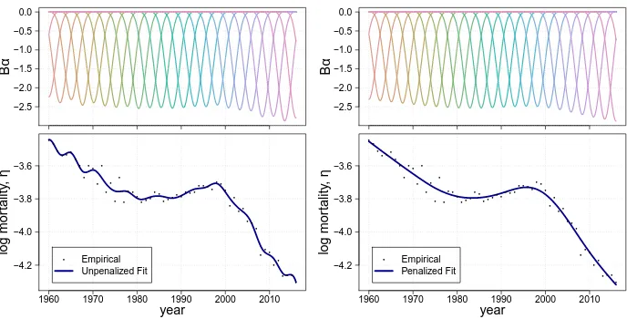
whereBarekequally spacedB-spline bases: bell-shaped curves composed of smoothly joined polynomial pieces of degree q. In the following we will use cubicB-splines, q = 3. The positions on the horizontal axis, where the pieces come together, are called “knots.” Details onB-splines and related algorithms can be found in de Boor (1978), and examples ofB-spline bases are provided on the top panels in Figure 1.
Figure 1: Unpenalized (left) and penalized (right)B-splines on Danish female mortality at age 70 from 1960 to 2016
B α −2.5 −2.0 −1.5 −1.0 −0.5 0.0 year log mor tality , η
1960 1970 1980 1990 2000 2010 −4.2 −4.0 −3.8 −3.6 ● ● ● ● ●● ● ● ● ●● ● ● ● ● ● ● ● ● ● ● ●● ● ● ● ●●●●● ● ● ● ● ● ●● ●● ● ● ● ●● ●● ● ● ● ● ● ● ● ● ● ● ● Empirical Unpenalized Fit B α −2.5 −2.0 −1.5 −1.0 −0.5 0.0 year log mor tality , η
1960 1970 1980 1990 2000 2010 −4.2 −4.0 −3.8 −3.6 ● ● ● ● ●● ● ● ● ●● ● ● ● ● ● ● ● ● ● ● ●● ● ● ● ●●●●● ● ● ● ● ● ●● ●● ● ● ● ●● ●● ● ● ● ● ● ● ● ● ● ● ● Empirical Penalized Fit
A penalized version of the iteratively reweighted least squares (IRLS) algorithm (McCullagh and Nelder 1989) is sufficient for estimating coefficientsα∈Rk:
(B0W B˜ +P) ˜α=B0W˜ z˜, (6)
wherez˜= (y−e∗µ˜)/e∗µ˜+ ˜ηis the working dependent variable.
The tilde symbol and∗denote current approximations to the solution and element-wise product, respectively.W˜ is a diagonal matrix of weights,W˜ =diag(e∗µ˜).
The only difference from the standard procedure for fitting a Generalized Linear Model (GLM) withB-splines as regressors is the modification ofB0W B˜ by a penalty factor given by
P =λD0D, (7)
where the matrixDconstructs differences in the coefficients over either ages or years. As examples, when we have only six coefficients and we use second-order differ-ences,Dis given by:
D=
1 −2 1 0 0 0
0 1 −2 1 0 0
0 0 1 −2 1 0
0 0 0 1 −2 1
When using a standardP-spline approach, the choice of the order of difference is crucial only for forecasting (cf. Section 2.1). Second-order difference will be used in the following: The smoothing parameterλregulates the trade-off between goodness of fit and effective dimension used in the model. On the one hand, higher values will lead to a higher penalty term and, consequently, smoother fitted values. On the other,λ= 0results in a straightforward GLM estimation withB-splines as regressors.
Figure 1 presents theP-splines logic applied to a one-dimensional example: Dan-ish females aged 70 from 1960 to 2016. On the top panels we havek = 25B-splines multiplied by associated coefficients that determine the height of eachB-spline. The bot-tom panels present empirical and estimated log mortality. On the left panels we have the outcomes from a simple GLM estimation (λ= 0). The right panels show the penalized version in which the coefficients are forced to change smoothly. The heights of the asso-ciatedB-splines therefore do not show wiggling behavior and, consequently, neither do the fitted values.
Our aim is to model and forecast mortality over both age and time, so we need to set up a P-splines model in a two-dimensional setting. For the purpose of regression, we arrange the complete matrices as a column vector, that is, y = vec(Y)ande = vec(E). Then we can directly use Equation (6) to estimate coefficients over age and years by generalizing both the basis and the penalty term.
LetBa,m×kaandBt1,n1×kt1be theB-splines over ages and years, respectively.
The regression matrix for our two-dimensional model is given by
B=Bt1⊗Ba, (9)
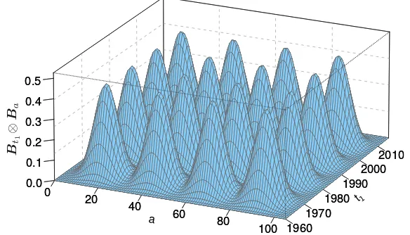
where⊗denotes the Kronecker product of two matrices. Following the same idea as for the one-dimensional case, we will use a relatively large number of equally spaced B-splines over both domains (ka = 24,kt1 = 14). Figure 2 shows a subset of the Kronecker
product basis for ages 0–105 and years 1960–2016. The age–year grid is populated by a dense set of overlapping hills that are placed at regular intervals as in an “egg carton.” Associated with each hill we will have a coefficient that will determine the height of its hill. Generalizing in 2D the concept illustrated in Figure 1, the fitted surface will be the sums of these two-dimensional heights.
Concerning the 2D generalization of the penalty term, from the definition of the Kronecker product, Currie, Durb´an, and Eilers (2004) show thatαcan be independently penalized over ages and years. LetDaandDt1 be the difference matrices acting on the
two domains. A two-dimensional penalty is given by
P =λa(Ikt1 ⊗D
0
aDa) +λt1(D
0
t1Dt1⊗Ika) , (10)
whereλa andλt1are the smoothing parameters used for age and year, respectively. Ika
Figure 2: A subset of two-dimensional Kronecker product cubicB-spline basis
a
0 20
40 60
80 100
t
19601970 19801990
20002010 0.0
0.1 0.2 0.3 0.4 0.5
0 20
40 60
80 100 19601970
19801990 20002010 0.0
0.1 0.2 0.3 0.4 0.5
1
By changingλaandλt1, smoothness can be tuned to balance smoothness and model
fidelity. In the followingλa andλt1 will be selected by minimizing the Bayesian
Infor-mation Criterion (BIC, Schwarz 1978) that penalizes model complexity more heavily and is more suitable for mortality data (Camarda 2008; Currie, Durb´an, and Eilers 2004).
As in the one-dimensional setting,B-splines provide enough flexibility to capture surface trends. The additional penalty reduces the effective dimension, leading to a
wiselyparsimonious model with a smoothed fitted surface. The advantage of using
two-dimensionalP-splines lies also in the fact that different smoothing parameters can be chosen over ages and years, leading to considerable model flexibility. Furthermore,P -splines in 2D can be embedded in the class of Generalized Linear Array Models, saving computational time and reducing storage problems in the estimation of the model (Currie, Durb´an, and Eilers 2006).
2.1 Forecasting withP-splines
In the original paper by Currie, Durb´an, and Eilers (2004), forecasting is treated as a missing-value problem and the smooth surface is simply extrapolated into future years. Keeping the same age range and forecasting over the years, we augment data andB-spline bases as follows:
˘
whereY2andE2arem×n2matrices filled with arbitrary future values. In this paper,
the completeB-spline basis over years will extend the original basis with an additional eightB-splines.
Finally, let us denote by1m×n1 an all-ones matrix over ages and firstn1observed
years. Similarly0m×n2 is a zero matrix over ages and futuren2 years. If we define a
weight matrixV:
V =diag(vec(1m×n1 :0m×n2)) , (11)
we can adapt the algorithm in (6) as follows:
( ˘B0VW˜ B˘+P) ˜α= ˘B0VW˜ z˜, (12)
withz˜ = V( ˘y−e˘∗µ˜)/e˘∗ µ˜ + ˜η. The penalty is also augmented to account for future years by difference matricesDa andDt1+t2. This unified structure allows us to
simultaneously model and forecast mortality. Moreover, the structure ofV makes it clear that, first, we use all observed data, and second, we assume nothing about the future, i.e., weights equal to one for the observed years and zero for the forecast horizon.
It is noteworthy that the form of the penalty determines the form of the forecast. Whereas the order of the penalty is negligible in the model section, it has a crucial role in the forecasting section. As suggested by Currie, Durb´an, and Eilers (2004), second-order differences inDt1+t2 are preferable because the forecast coefficients will be
approxi-mately linear over the future years, and this choice is more appropriate when working with mortality data. However, this aspect will lose its relevance when prior demographic knowledge is incorporated into the model (cf. Section 3).
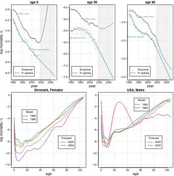
Figure 3 presents the outcomes of a two-dimensionalP-splines approach in model-ing and forecastmodel-ing mortality data for Danish females and US males. The top panels show empirical and fitted as well as forecast trends for selected ages (0, 50, 80). Concerning estimation on observed data,P-splines show a rather good fit, though unsmooth patterns are visible around age 10 in both populations (bottom panels in Figure 3). Nevertheless, an odd mortality increase in future years is visible for some ages in the US male data, and the forecast mortality improvement at age 80 for Danish females is probably too fast. These outcomes are obviously implausible given the observed mortality trends of the past years. The bottom panels in Figure 3 mirror the above mentioned results from a different perspective. For the future years, mortality age profiles are obviously improbable given the knowledge we already have on the phenomenon: Unreasonable wiggling behavior is evident from age 20 onward in both populations. This outcome can be seen as a conse-quence of a low smoothing parameter selected by the BIC for the age domain. A smallλa
Figure 3: Empirical, model and forecast mortality. Two-dimensional
P-spline approach. Selected ages over years (top panels) and selected years over ages (bottom panels)
log mor tality , η year age 0
1960 1980 2000 2020 2040 −6.5 −6.0 −5.5 −5.0 −4.5 −4.0 −3.5 ● ●●●●●● ●● ●● ● ●●● ● ● ●● ●● ●● ●●● ●●●● ●● ●● ● ● ●●●●●●●●●●●●●● ● ●●●●●● ●● ● ●●● ● ● ● ● ●● ●● ●● ● ● ● ● ● ●● ●● ● ● ● ●● ●● ● ●● ● ● ● ● ● ●● ●● ● ●● ● ● ● ● ●● ●●● ● ● Empirical P−splines Denmark, females USA, males year age 50
1960 1980 2000 2020 2040 −7.5 −7.0 −6.5 −6.0 −5.5 −5.0 −4.5 ●●●●●●●
●●●●●●●●● ●●● ●● ● ●●●●●●●● ●●●●●● ● ●●●●● ●●●●●●● ●●●●●●●● ●● ●● ● ●●● ● ● ● ●● ● ●●● ●● ● ● ● ● ● ● ● ● ● ● ●● ● ●● ● ● ●● ● ● ● ● ● ● ● ●●● ● ● ●● ● ●● ● ● ● Empirical P−splines Denmark, females USA, males year age 80
1960 1980 2000 2020 2040 −4.0 −3.5 −3.0 −2.5 ● ●● ● ●●●● ●● ●●●● ● ●● ●● ●●● ●●●●●●● ●●● ● ● ●●● ●●●● ●● ● ●● ● ●● ●●● ●●●●● ● ● ● ●● ●● ● ● ●●● ● ● ● ●● ● ● ● ●●●● ●●● ● ● ●● ●●●● ● ●●●● ●●● ● ● ●●●●●● ●● ● ● ● ● ● Empirical P−splines Denmark, females USA, males age log mor tality , η Denmark, Females
0 20 40 60 80 100
−12 −10 −8 −6 −4 −2 0 ● ● ● ● ●●● ● ● ●● ● ● ● ●● ●● ●●●● ● ●● ●● ● ● ● ● ●● ● ●● ● ●●●●●●●● ●●● ●●● ●●● ● ● ●●● ●●● ●●●● ●● ●● ●●●●●● ●● ●●●● ●● ●●●● ●●●●●●●● ●●● ● ● ● ● ● ● ● ● ● ● ● ● ● ● ● ● ●● ●●●● ● ● ● ● ● ● ●●● ●● ●● ●● ●● ● ● ●●●●● ●● ●●●● ●●●● ●●● ●●●●●● ●●●● ●●●● ●●● ●●●● ●●●●● ●●● ●●● ●●●●● ●● ●●●● ●● ● ● ● ● ● ● Model 1960 1990 Forecast 2020 2050 age USA, Males
0 20 40 60 80 100
−12 −10 −8 −6 −4 −2 0 ● ● ● ● ● ●● ●●●●●● ●● ● ●● ●●●●●●●●●●●●●●●●●●●● ●●●●●● ●●●● ●●●●●● ●●●●● ●●●●● ●●●●●● ●●●● ●●●●● ●●●●● ●●●●●●●●●●●●● ●●●●●● ● ● ● ● ● ● ● ● ●●●●●●● ●● ● ● ● ●●●●●●●●● ●●●●●●● ●●●●●●●●● ●●●● ●● ●●●●●●● ●●● ●●●● ●●●●●●●●●● ●●●● ●●●● ●●● ●● ●●●● ●●●● ●●●●●●●●●●●●● ● ● Model 1960 1990 Forecast 2020 2050
3. The
CP
-spline model
In the last section, we noted that several issues may occur when two-dimensionalP -splines are applied without any demographic consideration in a plain data-driven ap-proach. Specifically, we need to deal with infant mortality preserving smoothness in the following ages. Moreover, previous outcomes call for inclusion in forecast years of prior knowledge on typical mortality age profiles and time trends.
3.1 Addressing infant mortality
The first year of life is usually treated in a different manner when life tables are con-structed (Chiang 1984). Therefore, we decided to follow this practice by modifying the basis related to the age domain. The new basis will then be:
B0a=
1 01×ka
0(m−1)×1 Ba
, (13)
whereBais now a(m−1)×kamatrix ofB-splines.
Moreover we replace the first cell inDawith a zero, which implies that infant
mor-tality is not connected with variation in subsequent coefficients. In other words, we sep-arate development of infant mortality from the remaining ages.
Using this new basis and a new penalty ensures that a single and specialized co-efficient will be attached to infant mortality values. In a one-dimensional setting, this additional coefficient will be exactly the log of death rates at age 0. In a two-dimensional framework, we allow for a smooth change in infant mortality over time.
On the one hand, we increase the number of coefficients in the model. On the other, we allow a certain freedom in describing mortality at age 0 via its specific series of co-efficients over years. This ensures that the smoothness of the surface from age 1 onward will not be affected by the evident disruption due to infant mortality.
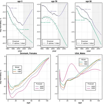
Figure 4 shows the outcomes for our Danish and US datasets when mortality levels at age 0 are explicitly considered. Although the forecast trends are still unreasonable, especially for US males, considering infant mortality as a peculiar phenomenon helps to improve goodness of fit during the observed period: BIC reduces from 79,308 to 34,795 for US males and from 8,135 to 7,701 for Danish females. The specifically optimized smoothing parameter for the age domain (λa) becomes larger with respect to the
Figure 4: Empirical, model and forecast mortality. Two-dimensional
P-spline approach including a specialized coefficient for infant mortality. Selected ages over years (top panels) and selected years over ages (bottom panels)
year log mor tality , η age 0
1960 1980 2000 2020 2040 −6.5 −6.0 −5.5 −5.0 −4.5 −4.0 −3.5 ● ●●●●●● ●● ●● ● ●●● ● ● ● ● ●● ●● ●●● ●●●●● ● ●● ● ● ●●●●●●●●●●●● ●● ● ●●●●●● ●● ● ●●● ● ● ● ● ●● ●● ●● ● ● ● ● ● ●● ●● ● ● ● ● ● ●● ● ●● ● ● ● ● ● ●● ●● ● ●● ● ● ● ● ●● ●●● ● ● Empirical P−splines + Infant
Denmark, females USA, males
year
age 50
1960 1980 2000 2020 2040 −7.5 −7.0 −6.5 −6.0 −5.5 −5.0 −4.5 ●●●●●●●
●●●●●●●●● ●●● ●● ● ●●●●●●●● ●●●●●● ● ●●●●● ●●●●●●● ●●●●●●●● ●● ●● ● ●●● ● ● ● ●● ● ●●● ●● ● ● ● ● ● ● ● ● ● ● ●● ● ●● ● ● ●● ● ● ● ● ● ● ● ●● ●● ● ●● ● ●● ● ● ● Empirical P−splines + Infant Denmark, females
USA, males
year
age 80
1960 1980 2000 2020 2040 −4.0 −3.5 −3.0 −2.5 ● ●● ● ●●● ● ●● ●●●●● ●● ●● ●●●●●●●●●● ●●● ● ● ●●● ●●●● ●● ● ●● ● ●● ●●●●● ●●● ● ● ● ●● ● ● ● ● ●●● ● ● ● ●● ● ● ● ●●●● ●●● ● ● ●● ●●●●● ●●●● ●●● ● ● ●●●●●● ●● ● ● ● ● ● Empirical P−splines + Infant Denmark, females USA, males age log mor tality , η Denmark, Females
0 20 40 60 80 100
−10 −8 −6 −4 −2 0 ● ● ● ● ●●● ● ● ●● ● ● ● ●● ●● ● ● ●● ● ●● ●● ● ● ● ● ●● ● ● ● ● ●●●●● ●●●●●● ●●● ●●● ● ● ● ●●●● ● ●●●●●● ● ●●●●●●● ●● ● ●●●●● ●● ●●●● ●●●●●● ● ●● ● ● ● ● ● ● ● ● ● ● ● ● ● ● ● ● ●● ●●●● ● ● ● ● ● ● ●●● ●● ●● ●● ● ● ● ● ●●●●● ●● ●●●● ●●●● ●●● ●●●●● ●●●●● ●●●● ●●● ●●● ●●●● ●● ● ●●●● ●●●● ●●●● ●●● ●●● ● ● ● ● ● ● Model 1960 1990 Forecast 2020 2050 USA, Males age
0 20 40 60 80 100
−10 −8 −6 −4 −2 0 ● ● ● ● ● ●●●● ●●●●● ● ● ●● ●●●●●●●●●●●●●●●●● ●●● ●●●● ●●● ●●●●●●● ●● ●●●●● ●●●●● ●●●●●● ●●●● ●●●●●● ●●●● ●●● ●●●●●●●●●●●●●●●●● ● ● ● ● ● ● ●●●●●●●● ● ● ● ● ● ●●●●●●●● ●●●●●●●●●●●●●●● ●●●●●●●● ●●●●●●● ●●● ●●●● ●●● ●●●●● ●●● ●●● ●●●● ●●●●● ●●●● ●●●● ●●●●●●●● ●●●●● ● ● Model 1960 1990 Forecast 2020 2050
3.2 Enforcing mortality patterns over age and time
As we have seen in Section 2.1, the originalP-spline approach is purely data-driven and the extrapolated trends are based on the last estimated coefficients solely constrained by a certain amount of smoothness. However, following Gompertz (1825), demographers started observing well-defined regularities in the shape of mortality over ages. Moreover, past mortality trends present a certain predictability that must guide any model. It would be unreasonable to disregard information on mortality patterns over ages and time in a forecasting method.
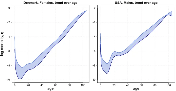
Regarding the age dimension, Figure 5 shows the 95% confidence interval over age based on the mortality surface, smoothed byP-splines with the additional specialized coefficient for infant mortality (cf. Section 3.1). A rather stable mortality behavior over ages is evident. In general, at infant ages, mortality decreases steeply, dropping rapidly within the first few years (Levitis 2011). A minimum is commonly reached at about ages 10–15. Afterward, especially for men, mortality rates show a hump at young adult ages (Goldstein 2011; Remund 2015). Mortality then rises exponentially after approximately age 30 and levels off at ages above 80 (Preston 1976; Thatcher, Kannisto, and Vaupel 1998).
Figure 5: 95% pointwise confidence intervals of mortality age profiles from fitted two-dimensionalP-splines approach
age
log mor
tality
,
η
Denmark, Females, trend over age
0 20 40 60 80 100
−10 −8 −6 −4 −2 0
age
USA, Males, trend over age
0 20 40 60 80 100
−10 −8 −6 −4 −2 0
Note: Model includes a specialized coefficient for infant mortality. Danish females (left panel) and US males (right panel), ages 0–105, years 1960–2016.
period without modifying fitted values which are based on observed and past data. Instead of borrowing mortality profiles from model life tables or parametric models, we constrain forecast age profiles lie within the 95% confidence interval of the fitted age profiles.
Since we aim to carry out our analysis referring to the mortality shape and regardless of its level, our constraints must be based on the relative derivatives of the age mortality profile, commonly named rate of aging. Given the estimated linear predictorηˆ =Bαˆ, the rate of aging for each year can be computed by a linear combination of a modified version of theB-splines and the estimated coefficients:
∂ ∂aµˆ
ˆ
µ =
∂
∂aln( ˆµ) =
∂
∂aηˆ=D
t1
a αˆ, (14)
where the matrixDt1
a computes the first difference of the estimated coefficients for each
year and simultaneously multiplies them byB-splines of lower degree. In the formula,
Dt1
a =Bt1⊗Ca, (15)
where
Ca = 1
h
q−1Bν
a−
q−1Bν−1
a
, (16)
withh,qandν being knot distance, degree, and positions of the originalB-spline basis,
Ba.
In this way, using directly estimated coefficients, we can compute the instantaneous rate of aging over all ages and for each year. This allows us to modify the algorithm in (12) for incorporating possible constraints. Moreover, when working on smooth mor-tality surfaces, estimated relative derivatives over age will not show the wiggling behavior produced by simple differentiation of observed death rates.
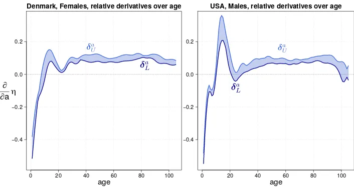
Figure 6 presents 95% confidence intervals of the instantaneous rate of aging over all ages above 0 for Danish females and US males. We denote byδaLandδUa the lower and upper bounds of these confidence intervals, respectively.
For better readability of the graph, relative derivatives for infant mortality are not displayed. A steep decrease in mortality at age 0 will enormously expand the limits of the ordinate of the associated rate of aging. Specifically, the 95% confidence interval of the relative derivatives with respect to age 0 is[−2.76,−2.39]for Danish females and
[−2.82,−2.56]for US males.
In Figure 6 we can read the mortality age patterns of our data without referring to their level. In general, values above zero correspond to mortality increase and, conversely, ages with mortality reduction coincide with negative values of the rate of aging.
parameter in the Gompertz model,α2in Equation (4). However, we do not predefine a
constant rate of aging for adult mortality, and can are also capture a possible leveling-off of mortality at oldest old ages. See the declining relative derivatives above age 80.
Figure 6: 95% pointwise confidence intervals of relative derivatives of force of mortality with respect to age, i.e., rate of aging,(δa
L,δ a
U). Fitted
values computed from fitted two-dimensionalP-splines approach
age
Denmark, Females, relative derivatives over age
∂ ∂aη
0 20 40 60 80 100
−0.4 −0.2 0.0 0.2
age
USA, Males, relative derivatives over age
0 20 40 60 80 100
−0.4 −0.2 0.0 0.2
Note: Shown only for ages 1–105. Model included a specialized coefficient for infant mortality. Danish females (left panel) and US males (right panel), ages 0–105, years 1960–2016.
The rate of aging also shows clear sex differences in young adult mortality: Danish females present a U-shape pattern about age 20 that is much less pronounced than for US males. This latter population also reaches relative derivatives equal to zero around age 25, which means a corresponding constant mortality. This sex difference points out the young adult excess mortality that is particularly evident for males (see Figure 5). In both populations, the decreasing mortality trend during childhood is clear: The associated rate of aging shows a steeply increasing pattern with negative values.
Concerning time trends, we can compute relative derivatives with respect to time as we did for the age domain:
∂ ∂t1µˆ
ˆ
µ =
∂ ∂t1
ln( ˆµ) = ∂
∂t1
ˆ η=Dt1
t1αˆ. (17)
Again matrixDt1
t1 computes first difference of estimated coefficients by
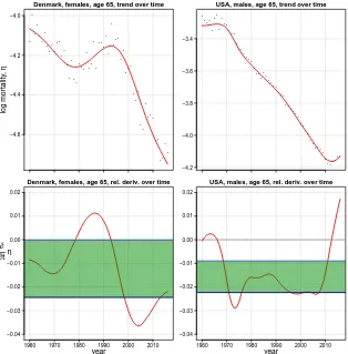
fluctuates more than the age profile, as one can see by looking at a particular age (65) for both Danish females and US males in Figure 7. Whereas the trend is generally smooth and downward, there are periods of mortality increase: during the 1980s for Danish fe-males and the most recent years for US fe-males. Mortality stagnation in US fe-males is also evident during the 1960s.
Figure 7: Empirical and smooth log mortality for age 65 over time (top panels) and associated rate of change (bottom panels). Horizontal blue lines depict 50% confidence intervals of the rate of change. Fitted values computed by two-dimensionalP-splines approach
log mor tality , η ● ● ● ● ● ● ● ● ● ● ● ●● ● ● ● ● ● ● ● ● ● ● ● ● ● ● ● ● ● ● ● ● ● ● ●● ● ● ● ●● ● ● ● ● ● ● ●● ● ●● ●● ● ● −4.6 −4.4 −4.2 −4.0
Denmark, females, age 65, trend over time
● ● ●● ● ● ● ● ● ●● ● ● ● ● ● ● ● ● ●● ● ● ● ● ● ● ●● ● ● ● ● ● ●● ● ●● ● ● ● ● ● ● ● ● ● ● ● ● ● ● ●● ●● −4.2 −4.0 −3.8 −3.6 −3.4
USA, males, age 65, trend over time
year
1960 1970 1980 1990 2000 2010 −0.04 −0.03 −0.02 −0.01 0.00 0.01 0.02
Denmark, females, age 65, rel. deriv. over time
∂ ∂t η
year
1960 1970 1980 1990 2000 2010 −0.04 −0.03 −0.02 −0.01 0.00 0.01 0.02
USA, males, age 65, rel. deriv. over time
These features are immediately visible in the associated relative derivatives with respect to time for mortality at age 65 in both populations (bottom panels in Figure 7), which express mortality improvement over time regardless of the actual level. Likewise for the rate of aging, negative values correspond to downward mortality trends, which represents the majority of the observed relative derivatives for this specific age. Positive values are observed when mortality stagnates and/or deteriorates.
Although values for mortality rate of change over time are smaller than the observed rate of aging, variation is wider: Every mortality fluctuation over time even minor -is amplified in the associated relative derivatives. Note, for example, the time trend in US males aged 65 in the most recent years: A rather small estimated increase translates into a disproportionate jump in the rate of change (right panels in Figure 7). This is a well-known issue in statistics: Derivatives will always show undersmooth behavior with respect to the associated estimated function (Erickson, Fabian, and Marik 1995).
On the one hand, we aim to constrain future mortality developments to lie within observed mortality rates-of-change. On the other, we intend to avoid in future years the peculiar past mortality trends that we assume to be solely due to specific and unlikely events. For this reason we decide to use only 50% confidence intervals of the observed mortality rate of change, i.e., the interquartile range of past experienced mortality devel-opment.
We recommend the interquartile range based on several experiments conducted on numerous populations from the Human Mortality Database (2019) (not shown here). However, it is important to note that this value (50%) is simply a way to express the forecaster’s prior knowledge of how past mortality should inform future development. As a result, different attitudes toward the future or the peculiar mortality history of a spe-cific population may guide forecasters to different values in computingδt1
L andδ
t1
U. In
the Supplementary Materials C we evaluate this choice for Danish females and US males. Outcomes do not change markedly, as long as extreme mortality fluctuations over time are not considered. Moreover, we present an out-of-sample forecast exercise which could be eventually used to select population-specific percentages for computingδt1
L andδ
t1
U.
The horizontal green stripes in the bottom panels of Figure 7 depict the 50% confi-dence intervals of the observed mortality rate of change for age 65 in both populations.
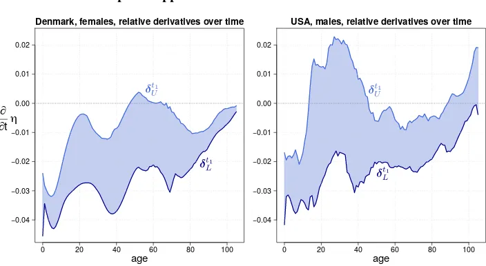
Figure 8 shows the 50% confidence intervals of the relative derivatives of the force of mortality with respect to time for each age. The lower and upper levels of these confi-dence intervals are denoted byδt1
L andδ
t1
U, respectively.
In Figure 8 we can easily see which ages have experienced greater improvements (larger negative values) as well as with greater variations in terms of observed mortality changes (broader confidence bounds).
time trends expressed by estimated values and portrayed in Figures 6 and 8. Hence, we propose the Constrained Penalized spline (CP-spline) model.
Figure 8: 50% pointwise confidence intervals of relative derivatives of force of mortality with respect to time for each age, i.e., age-specific rate of change. Fitted values computed from fitted two-dimensional
P-splines approach
age
∂ ∂tη
0 20 40 60 80 100
−0.04
−0.03
−0.02
−0.01 0.00 0.01 0.02
Denmark, females, relative derivatives over time
age
0 20 40 60 80 100
−0.04
−0.03
−0.02
−0.01 0.00 0.01 0.02
USA, males, relative derivatives over time
Note: Model included a specialized coefficient for infant mortality. Danish females (left panel) and US males (right panel), ages 0–105, years 1960–2016.
Although specific values are suggested for computingδ, forecasters can adapt the model to their needs and to prior knowledge about future mortality development. In gen-eral, the lower the percentages in estimating the vectors ofδ, the closer future mortality will be to mean age patterns and time trends, as observed in past years. In other words, extremely low percentages forδlead to a fixed age profile, along with an invariant age-specific rate of mortality improvement, i.e., something similar to the Lee–Carter model, but with a nonlinear time index based on the amount of smoothness. Conversely, large confidence levels leads to an extremely flexibleCP-spline model without much prior knowledge about future mortality, i.e., a plainP-splines approach. Additionally, differ-ent levels of mortality improvemdiffer-ent can be set for differdiffer-ent ages, making the model highly flexible. Finally, the choice of the percentage for computingδa
LandδaU is less important
than forδt1
L andδ
t1
U. Derivatives are computed on previously smooth rate values, and
val-ues higher than 95% for constraining the age profile will only slightly modify the final outcomes.
We must warn the forecaster on two important issues. First, allowing high flexibility may lead to unreasonable outcomes (see Figure 3), whereas the other, a rigid model will forecast patterns that slavishly reproduce the structure of the model in future years. Second, recommended levels for computingδ inCP-splines should be adopted with care: Although they have been tested for many datasets in the Human Mortality Database (2019), specific populations might need distinct confidence levels to either account for or neglect unique patterns over age and/or years.
3.2.1 Incorporating prior knowledge into the model
Once the constraints are set, we retain them for all years by augmenting the values inδ
over both dimensions:
ga
L = 1n1+n2⊗δ
a L
ga
U = 1n1+n2⊗δ
a U
and g
t
L = 1n1+n2⊗δ
t1 L
gt
U = 1n1+n2⊗δ
t1 U
(18)
We enforce our shape constraints by adding asymmetric penalties within the system introduced in (12):
( ˘B0VW˜ B˘ +P+Pa+Pt) ˜α= ˘B0VW˜ z˜+pa+pt, (19)
where
Pa = PLa+PUa
Pt = PLt+PUt and
pa = paL+paU
pt = ptL+ptU . (20)
As an example, we present the penalty terms for the lower bounds over ages. The other terms are constructed in a similar fashion. In formulas
Pa
L = κD
t1+t20
a diag(sv˜La)D
t1+t2 a
pa
L = κD
t1+t20
a diag(sv˜La)g
a L
withvaL =
(
0 if Dt1+t2 a α˜ >gLa 1 if Dt1+t2
a α˜ <gLa ,
andsis a 0/1 vector equal to 1 when the constraint is to be applied (future years). Note that, being asymmetric, these penalties act on both the left and right sides of the system of equations, and values inva
L,v a
U,v
t
L andv
t
U are computed iteratively.
In other words, for each new value ofα˜ during the iteration (19), the shape penalties exert an influence only when the shape constraint is violated. The size ofκregulates how strictly the constraints are enforced. In this paper, we choseκ = 104, which is
values as expressed in the roughness penaltyP. More details on asymmetric penalties and their statistical properties can be found in Eilers (2005) and Bollaerts, Eilers, and van Mechelen (2006).
3.2.2 Confidence intervals by bootstrap
No forecasting method can be completely satisfactory without an estimation of the un-certainty affecting the forecast quantities. Estimation of confidence intervals is thus par-ticularly necessary. It is noteworthy that CP-splines intrinsically constrain future log mortality within defined ranges of possible outcomes, and these constraints hold within the estimation of the associated standard errors. The consequences are twofold: On the one hand, confidence intervals for future years will always contain values that lie within the defined shape constraints and, on the other, the interval will often be narrower with respect to alternative methods. Relaxation of the shape constraints by smaller values ofκ and larger confidence levels for computingδ, or accounting for the overdispersion that is generally found in mortality data may mitigate this drawback. These generalizations of the current approach will be avenues for future research.
In practice, without shape constraints, plain two-dimensionalP-splines are a straight-forward extension of a regression model, and methods for computing the covariance ma-trix and associated standard errors can be borrowed from regression theory. However, with ourCP-spline model, we depart from this setting with the inclusion of asymmetric penalties in the system of equations.
In the absence of analytical solutions for the estimation of uncertainty in our model, we opt for confidence intervals constructed via a bootstrap approach. We are thus able to combine all sources of uncertainty in the model and simultaneously compute confidence intervals for summary measures, which are complicated nonlinear functions of the esti-mated coefficients. Details on bootstrap methods in general can be found in Efron and Tibshirani (1993). While bootstraps have been used by Brouhns, Denuit, and Van Keile-gom (2005) and Koissi, Shapiro, and H¨ogn¨as (2006) in the Lee–Carter context, Ouellette, Bourbeau, and Camarda (2012) have adapted this methodology to a two-dimensionalP -spline model.
Following Koissi, Shapiro, and H¨ogn¨as (2006) and Ouellette, Bourbeau, and Ca-marda (2012), we carried out a residual bootstrap of our fitted model. Specifically, de-viance residuals are the standard measures to assess the discrepancy between empirical and fitted data (McCullagh and Nelder 1989: 39–40):
r= sign(y−yˆ) s
2
yln
y
ˆ y
−y+ ˆy
. (21)
is well specified). Hence, we sample from them (with replacement) an entire new set of residuals r(b) called the bootstrapped residuals. Replacing deviance residuals r with
bootstrapped residualsr(b)in (21) and rearranging the equation leads to
ˆ
y−yln( ˆy) +r(2b)+y−yln(y) = 0 . (22)
Givenr(b)and actual deathy, equation (22) can be solved numerically with respect
toyˆ, thus obtaining a new matrix of bootstrapped deathsyˆ(b). Together with the original
exposurese, we can estimate the proposedCP-spline model on the bootstrapped deaths
ˆ
y(b), obtaining new bootstrapped coefficientsαˆ(b).
The procedure described above, starting with the residual sampling step, was re-peated 1,000 times. This led to a bootstrapped distribution of constrained and penalized coefficients. From this distribution, we extract empirical percentiles and compute confi-dence intervals for force of mortalityµand linear predictorη, as well as for any desirable summary measure, e.g., life expectancy at birth.
Whereas common approaches focus on the variability in the (univariate) time index (see both Lee–Carter and Hyndman–Ullah variants), residual bootstrap incorporates the variability from all model parameters. This approach is more suitable in a nonparamet-ric framework, and it allows us to account for uncertainty due to the Poisson stochastic process in (2), i.e., larger populations would tend to have narrower confidence intervals in the fitting periods.
When we apply any distinct forecasting model we do not question uncertainty due to model misspecification. Similarly, within aCP-spline framework, we specify a cer-tain model structure: Values of optimized smoothing parameters and confidence levels for computingδare kept fixed in the bootstrapping procedure. However, unlike other approaches, complexity of the model structure is data-driven in the estimation procedure. See columns with effective dimension (ED) in Table A-1 and A-2 in Supplementary Ma-terials.
To sum up, a forecaster that intends to estimate and forecast mortality byCP-splines needs to adopt the following procedure:
1. Collect as in (1) deaths and exposures in two matrices over age and years;
2. Estimate a two-dimensionalP-spline model over the observed period with the al-gorithm in (6) and a specialized basis for infant mortality as in (13);
3. Optimize smoothing parameters in the penalty term (10);
4. Evaluate rate of aging and rate of change for each age using (14) and (17); 5. Portray previous relative derivatives as in Figures 6 and 8 to decide on level of
confidence for future rate of aging (δa
L,δUa) and rate of change (δ t1
L,δ
t1
U). Here,
6. Solve the system of equations in (19), which adds in the forecasting algorithm (12) the asymmetric penalty terms;
7. Carry out the residual bootstrap presented above to obtain confidence intervals of the fitted model.
Routines for running all previous steps and forecast mortality withCP-splines were implemented inR(R Development Core Team 2019). Available on the journal’s website are routines that do not require stringent package installations. In terms of computational time, for a single population, fitting the model takes about 20 seconds, and it takes less than 80 minutes to run the bootstrap procedure with 1,000 simulations (portable personal computer, Intel i5-6300U processor, 2.4 GHz×4 and 16 Gbytes random-access mem-ory). Concerning computer data storage, a file of about 125 MB can store theRworkspace with all outcomes for a single population.
4. Application
Figure 9 shows the outcomes of the proposed smooth constrained forecasting model. In order to better visualize uncertainty around estimated values, we portray outcomes by means offanplot(Abel et al. 2013). Colored bands are limited by 10% and 90% of the empirical percentiles.
Moreover, in this section, we compare the outcomes from the suggestedCP-splines with a variant of the Lee–Carter model. Specifically, we apply the Lee–Carter model estimated in a smooth setting as described in Delwarde, Denuit, and Eilers (2007). Both theCP-spline model and this Lee–Carter variant are embedded in a Poisson framework, and smoothing of the coefficients is ensured in both settings. Hence, differences between models will be solely due to differences in model structure.
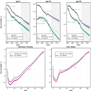
It is evident in Figure 9 how fitted values fromCP-splines follow empirical patterns adequately and forecast values fromCP-splines present reasonable trends over both ages and years. Specifically, there is no wiggling behavior because we enforce a specific shape via the asymmetric penalties, which also ensures no crossover of adjacent ages in the long term. Moreover, future mortality of US males no longer shows increasing trends.
Figure 9: Empirical, model and forecast mortality along with their bootstrapped distributions. Constrained Penalized spline model including a specialized coefficient for infant mortality. Estimates from a smooth Lee–Carter variant are given for comparative reasons log mor tality , η year age 0
1960 1980 2000 2020 2040 −7 −6 −5 −4 ● ●●●●● ●●● ●● ● ● ●● ● ● ●●●● ●● ●●● ●●●●● ● ●●● ●●●●●● ●●●●●●●●● ●●●●●●● ●● ● ●●● ● ● ● ● ●● ●● ●● ● ● ● ●●●●●● ● ● ● ●● ●● ● ●● ●●●● ● ●● ●● ● ●●● ● ● ●●● ●●● ● ● Empirical Smooth Lee−Carter CP−splines Denmark, females USA, males year age 50
1960 1980 2000 2020 2040 −6.5 −6.0 −5.5 −5.0 −4.5 ● ●●●●●● ● ● ●● ●●●● ● ●●● ●● ● ● ●●●● ● ●● ●●●●●● ● ●●●●● ●●●●●●● ● ●●●●●●● ●●●● ● ●●● ● ● ● ●● ● ●●● ●● ● ● ● ● ● ● ● ● ● ● ●● ● ●● ● ● ● ● ● ● ● ● ● ● ● ●●● ● ● ●● ● ● ● ● ● ● Empirical Smooth Lee−Carter CP−splines Denmark, females USA, males year age 80
1960 1980 2000 2020 2040 −3.5 −3.0 −2.5 ● ●● ● ●●● ● ●● ●●●●● ●● ●● ● ●● ● ●●●● ●● ●● ● ● ● ●●● ●●●● ●● ● ●● ● ●● ●●● ●●●●● ● ● ● ●● ● ● ● ● ●●● ● ● ● ●● ● ● ● ●●●● ●●● ● ● ●● ●●● ●● ●●●● ●●● ● ● ●●●●●● ●● ● ● ● ● ● Empirical Smooth Lee−Carter CP−splines Denmark, females USA, males age log mor tality , η Denmark, Females
0 20 40 60 80 100
−10 −8 −6 −4 −2 0 Smooth Lee−Carter CP−splines 2020 2050 age USA, Males
0 20 40 60 80 100
−10 −8 −6 −4 −2 0 Smooth Lee−Carter CP−splines 2020 2050
At first glance, the boundary of the confidence intervals in Figure 9 is extremely close to the fitted values in the observed period (1960–2016). This is mainly due to the large expected values in the Poisson distribution (2) which are the products of force of mortality and population exposure, remarkably large for US males. Consequently, we see relatively larger confidence bands at oldest ages over the years. In this area, high force of mortality is compensated by exposures with moderate counts. Similarly, slightly wider variability is observed at young ages (see pattern at age 20). This results from low force of mortality along with a large exposure population. The relatively larger uncertainty at age 0 is due to its peculiar treatment within the model: Smoothness is enforced only over time and therefore larger variability is expected. Moreover, variability increases for all ages the further we move toward future years.
In Figure 9 it is evident how the proposedCP-spline approach clearly outperforms the Lee–Carter model in fitting past trends: For US males, the deviance that measures goodness of fit in a Poisson setting is equal to 32,906 forCP-splines and 175,726 for the smooth Lee–Carter variant. For Danish females, the deviance is equal to 7,728 (12,831) forCP-splines (smooth Lee–Carter). A larger comparison with other forecasting meth-ods is available in the supplementary materials to this paper.
Concerning patterns for future years, the Lee–Carter model is not able to capture all observed mortality changes of the past decades, and its forecast trends are often unrea-sonable, i.e., a simple linear extrapolation of fitted values, which are a poor description of empirical trends. It is noteworthy that, although embedded in a smooth setting, the rigidity of the Lee–Carter structure leads to unsmooth fitted values. On the contrary, the proposed model does not suffer from this drawback and is able to accommodate diverse trends.
A direct consequence of these differences is visible in the age profiles in 2050 (bot-tom panels of Figure 9). Whereas the CP-spline model yields smooth and plausible future mortality age-patterns, the Lee–Carter produces unrealistic wiggling behavior of the age-profile in 2050 for both populations.
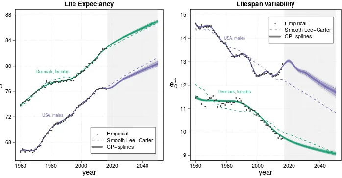
We decided to assess the performance of the proposedCP-spline model by means of two complementary summary measures. Life expectancy at birth is used as a classic measure of average lifespan. Lifespan variation describes differences in the length of life across members of a population and, among the large number of possible measures, we opt for the average number of life years lost at birth (Vaupel and Canudas-Romo 2003; Zhang and Vaupel 2009), commonly denoted bye†0. Easy to interpret as a potential increase in life expectancy at birth, this measure has already been used to evaluate the performance of mortality forecasts (Bohk-Ewald, Ebeling, and Rau 2017).
The results in terms of these summary measures are presented in Figure 10. As in the case of log mortality, theCP-spline model fits the development ofe0over the past years
rather well in both populations. The largest difference ine0between empirical and fitted
Figure 10: Empirical, model, and forecast values for life expectancy at birth (left panel) and a measure of lifespan variability (eee†0†0†0, right panel). Constrained Penalized spline model including a specialized coefficient for infant mortality
year
Life Expectancy
1960 1980 2000 2020 2040
68 72 76 80 84 88 e0 ●●●● ●●● ●●● ●●●● ●●● ●●● ●● ●●●●●●●●●●●●●●● ●●● ●●● ●● ●●● ●●● ●●●●●● ●●●●●●●●●●● ●●● ● ●● ●●●● ●●● ●●●●●● ●●●●● ● ● ●●●●● ●● ●●● ●● ●●●●●●●● Denmark, females USA, males ● Empirical
Smooth Lee−Carter
CP−splines
year
e0
Lifespan variability
1960 1980 2000 2020 2040
9 10 11 12 13 14 15 ●● ● ● ●●●● ●● ● ● ●●●● ●●● ●●● ● ●●● ●● ● ●●●●●● ●●● ●●● ●●● ● ● ● ●● ●●●● ● ●●●● ●●●●●● ● ●●●● ●● ●● ● ● ● ●●●●●●●●● ●●● ● ● ● ● ●●●●●●● ●● ●● ●●●● ●● ● Denmark, females USA, males ● Empirical
Smooth Lee−Carter
CP−splines
Note: Colored bands depict 80% of the empirical percentiles. Estimates from a smooth Lee–Carter variant are given for comparative reasons. Danish females and US males, ages 0–105, years 1960–2016, forecast up to 2050.
In 2050 the proposed method results in a life expectancy at birth of 86.97 years with a 95% confidence interval (86.66–87.30) for Danish females, and of 80.36 years for US males (79.88–80.92). We compare our results to those released by the United Nations in the 2019 World Population Prospects, medium variant (United Nations 2019). For Danish females, for the periods 2045–2050 and 2050–2055, the results provide a life expectancy at birth equal to 86.13 and 86.68, respectively. These values are slightly lower than our forecast 95% confidence intervals. On the contrary, we produce more pessimistic outcomes for US males: United Nations forecaste0equal to 81.40 and 82.17 for the two
periods, about 2050.
measures are also adequately described and forecast by the proposed model (not shown here).
Despite a similar final value in 2050, the development of future life expectancy at birth is different from that of the Lee–Carter model, which simply extrapolates a linear trend from erroneously estimated values. The proposedCP-spline model, on the other hand, is able to capture curved trends over time and consequently to provide more reliable forecasts.
Unlike the proposed approach, which is capable of reproducing all changes in lifes-pan variability measures, the Lee–Carter approach poorly estimates observed trends in e†0, and then linearly extrapolates its fitted values.
In the supplementary materials, we further assess the performance of the proposed model in additional ways. We compareCP-splines with alternative methods (Supple-mentary Material A), and we test stability with respect to the time window over which the model is estimated, an important and often neglected choice in all forecasting methods (Supplementary Material B).
Specifically, we present a large and detailed comparison study in whichCP-splines have been analyzed with five alternative forecasting methods: the mentioned smooth vari-ant of the Lee–Carter model (Delwarde, Denuit, and Eilers 2007); the Lee–Carter varivari-ants proposed Lee and Miller (2001) and by Booth, Maindonald, and Smith (2002), and two of the approaches proposed within a functional data framework by Hyndman and Ul-lah (2007). We model four countries (United States, Denmark, France, and Japan), both males and females, for the period 1960–2016 and forecast up to 2050. For the observed years, we assess goodness of fit (balanced with model complexity) using the Bayesian In-formation Criterion. In all datasets the proposedCP-splines outperformed the alternative approaches.
To evaluate the performance against observed mortality trends, we performed an out-of-sample forecast study. We estimate all models on the period 1960–2006, forecast up to 2016 and compare to observed values in 2005–2016. Models are compared using three different measures computed one0,e†0and the whole mortality surface (η). Given
Table 1: Root Mean Square Errors from the out-of-sample forecast exercise computed oneee000,ee0†
† 0 e†
0andηηη. Lower values (in bold) correspond to greater accuracy. Fitting period 1960–2006, forecast up to 2016 and compared to observed values in 2007–2016
CPCPCP-S LCsmo LM BMS HU HUrob
e0 0.154 0.203 0.184 0.200 0.369 0.302
e†
0 0.224 0.229 0.204 0.200 0.313 0.276
USAf
η η
η 0.079 0.128 0.123 0.123 0.103 0.086
e0 0.690 1.420 0.793 1.299 1.237 1.033
e†
0 0.235 0.850 0.658 0.708 0.516 0.248
DNKf
η η
η 0.324 0.420 0.367 0.373 0.344 0.328
e0 0.404 1.049 0.777 0.986 0.319 0.601
e†
0 0.105 0.317 0.505 0.455 0.298 0.126
JPNf
η η
η 0.121 0.287 0.241 0.265 0.123 0.122
e0 0.368 0.431 0.358 0.438 0.172 0.258
e†
0 0.047 0.263 0.244 0.267 0.101 0.048
FRAf
η η
η 0.107 0.180 0.157 0.157 0.120 0.109
e0 0.192 0.269 0.297 0.264 0.306 0.304
e†
0 0.349 0.614 0.570 0.600 0.469 0.399
USAm
η η
η 0.092 0132 0.126 0.128 0.110 0.099
e0 1.069 1.440 1.457 3.804 1.047 1.345
e†
0 0.308 0.247 0.409 0.861 0.097 0.250
DNKm
η η
η 0.358 0.372 0.427 0.809 0.364 0.373
e0 0.152 0.391 0.311 0.389 0.226 0.300
e†
0 0.095 0.088 0.092 0.098 0.260 0.196
JPNm
η η
η 0.104 0.154 0.163 0.168 0.101 0.097
e0 0.297 0.463 0.305 0.617 0.166 0.540
e†
0 0.081 0.130 0.089 0.160 0.205 0.053
FRAm
η η
η 0.101 0.209 0.455 0.433 0.134 0.138
Note: Populations: United States, Denmark, Japan, and France; females and males. Models:CP-splines (CP-S), smooth Lee–Carter (LCsmo), Lee-Miller (LM), Booth-Maindonald-Smith (BMS), Hyndman–Ullah (HU), and a robust version of Hyndman–Ullah (HUrob). Larger comparison is shown in the Supplementary Materials.
5. Conclusions
capture mortality developments over age and time, or too flexible to impose certain well-known structures in absence of observed data.
Among the rigid models, one can certainly list parametric models such as Gompertz and Heligman-Pollard. These models predefine a mortality law over age, and forecast estimated parameters will reproduce with a blind adherence these laws in future years. However, several Lee–Carter variants suffer from equivalent drawbacks describing all the mortality developments within a bilinear model and fixing an age-specific rate of mortality improvement. To free mortality models from rigid structures, nonparametric methods have been suggested. Superior in describing observed patterns, these approaches do not account for demographic knowledge in guiding forecast mortality developments.
Our study bridges the gap between these seemingly distant approaches. We enhance a powerful nonparametric statistical methodology, incorporating observed demographic information from the past years into the model. Under aP-spline approach we obtain good fit, flexibility, and smooth outcomes. Nevertheless, we show that a plain smoothing approach results in unreasonable outcomes when used to forecast mortality. This purely data-driven approach is not able to reproduce past mortality experience because it ex-trapolates last estimated trends with blind adherence. A certain amount of smoothness is the only restriction integrated into the model, and it is not sufficient when no data are available, as in the case for future years.
Thus, our proposal accomodates theP-splines approach, constraining future mor-tality to lie within trends estimated from observed data. We thus propose a Constrained Penalized spline (CP-spline) model. Initially, we consider infant mortality as a specific age and attach to age 0 a specialized coefficient. This improves the estimation of past trends but is insufficient to correct inconsistent trends in future years. Consequently, we also incorporate information about past mortality experience. Instead of working on ob-served log mortality, we operate in terms of rate of aging and rate of change over time. In practice, we enforce shape constraints by asymmetric penalties based on observed rel-ative derivrel-atives of the force of mortality with respect to age and time. Uncertainty on estimated and forecast quantities is then computed by a residual bootstrap approach. In this way we are able to simultaneously smooth past trends and forecast mortality in a sensible manner.
In the paper, we specified levels of confidence for rate of aging and rate of change aiming to constrain future mortality to observed shapes. These levels can be adapted to express diverse prior knowledge about future mortality for a distinct population and/or for specific ages. Specifically, our model might provide a means for guiding expert-based forecast approaches. Whereas it is hard to explicitly foresee future values for age-specific mortality rates, experts in the field may have more precise opinions on (un)feasible ranges of mortality improvements for ages, or groups of ages, looking to what has been observed in the past. This is obviously a population-specific procedure, and it will help to forecast populations that experienced exceptional patterns such as HIV epidemics, wars, and gen-eral mortality crises. We plan a gengen-eralization of the proposed CP-splines for these peculiar situations. Moreover, we envisage a large use of theCP-splines on all avail-able and comparavail-able mortality data. This will allow researchers to calibrate the choice of possible future age patterns and time trends based on broader past experiences, and eventually guide forecasters toward a more informed selection of possible constraints. In a Bayesian framework, and for forecasting cohort fertility, a similar approach was pro-posed by Schmertmann et al. (2014).
Specific cohort effects can be observed in certain populations and, in these situations, forecasters search for a procedure to incorporate these effects in the forecast horizon. Shape constraints over the diagonal of the mortality surface can be employed for accom-modating peculiar cohort behaviors without influencing neighboring cohorts. Similarly, the proposed model may provide a flexible and rigorous approach for deriving the age pattern of mortality given a predicted level of life expectancy and/or lifespan variability measures. We plan to extend our model along both lines.