EXPONENTIAL DOMINATION OF TREE RELATED GRAPHS
A. AYTAC¸1, B. A. ATAKUL2, §
Abstract. The well-known concept of domination in graphs is a good tool for analyzing
situations that can be modeled by networks. Although a vertex in the graph can exert influence on, or dominate, all vertices in its immediate neighbourhood, in some real world situations, this can be change. The vertex can also influence all vertices within a given distance. This situation is characterized by distance domination. The influence of the vertex in the graph doesn’t extend beyond its neighbourhood and even this influence decreases with distance. Up to the present, no framework for this situation has been put forward yet. The dominating power of the vertex in the graph decreases exponentially, with distance by the factor 1/2. Hence a vertexv can be dominated by a neighbour of v or by a number of vertices that are not too far fromv. In this paper, we study the vulnerability of interconnection networks to the influence of individual vertices, using a graph-theoretic concept of exponential domination number as a measure of network robustness.
Keywords: Graph vulnerability, Network design and communication, Domination, Ex-ponential domination number, Trees.
AMS Subject Classification: 05C40, 05C69, 68M10, 68R10
1. Introduction
Network designers attach importance of reliability and stability of a network. If the network begins losing communication links or processors, then there is a loss in its ef-fectiveness. This event is called as vulnerability of communication networks[11, 12]. The vulnerability of communication networks measures the resistance of a network to a disrup-tion in operadisrup-tion after the failure of certain processors and communicadisrup-tion links. Network designs require greater degrees of stability and reliability or less vulnerability in commu-nication networks.
Graph theory has become one of the most powerful mathematical tools in the analysis and study of the architecture of an interconnection network. It is well known that the underlying topology of an interconnection network is modeled by the graph. Throughout this paper, all graphs considered are simple and connected. Let G = (V, E) be a simple
1
Department of Math., Faculty of Science, Ege University, Bornova-Izmir,Turkey. e-mail: aysun.aytac@ege.edu.tr; ORCID: https://orcid.org/0000-0003-2086-8969. 2
Department of Comp. and Inst. Tech. Edu., Faculty of Education, A˘grı Ibrahim C¸ e¸cen University, A˘grı, Turkey.
e-mail: batay@agri.edu.tr; ORCID: https://orcid.org/BAA26021987.
§ Manuscript received: April 18, 2017; accepted: August 25, 2017.
TWMS Journal of Applied and Engineering Mathematics, Vol.9, No.3 cI¸sık University, Department of Mathematics, 2019; all rights reserved.
connected graph with a vertex setV =V(G) and an edge set E=E(G). For any vertex
v ∈ V(G), the open neighbourhood of v is N(v) = {u ∈ V(G)|uv ∈ E(G)} and closed neighborhood of v is N[v] =N(v)∪ {v}. The degree of v in G denoted bydeg(v), is the size of its open neighborhood. Thedistance d(u, v) between two vertices u and v in Gis the length of a shortest path between them. The diameter of G, denoted by diam(G) is the largest distance between two vertices inV(G)[13, 27].
Many graph theoretical parameters such as connectivity, toughness, integrity, binding number, domination number etc., have been used in the past to describe the stability of communication networks [2, 4, 5, 6, 7, 8, 9, 10, 24, 25, 26].
Domination in graphs is one of the concepts in graph theory which has attracted many researchers to work on it because of its many and varied applications in such fields as lin-ear algebra and optimization, design and analysis of communication networks, and social sciences and military surveillance [23]. A setS ⊆V(G) is a dominating set if every vertex inV(G)−S is adjacent to at least one vertex inS. The minimum cardinality taken over all dominating sets of G is called the domination number of G and is denoted by γ(G). Many variants of dominating models are available in the existing literature. The expo-nential domination number is one of these. It has been defined recently by Dankelmann et al. [16]. In their model, thedominating powerof a vertex decreases exponentially, with distance by the factor 1/2. Hence a vertexvcan be dominated by a neighbour ofvor by a number of vertices that are not too far fromv. Such a model could be used, for example, for the analysis of dissemination of information in social networks, where the impact of the information decreases every time it is passed on.
Let S ⊆ V(G). For each vertex u ∈ S and for each v ∈ V(G)−S, we define d(u, v) to be the length of a shortestu−v path in V(G)−(S− {u}) if such a path exists, and ∞ otherwise. If, for eachv∈V(G) we have
ws(v) =
P
u∈S1/2d(u,v)−1, if v /∈S
2, if v∈S
wS(v) ≥ 1, then S is an exponential dominating set. The smallest cardinality of an
exponential dominating set is the exponential domination number,γe(G) such a set is a
minimum exponential dominating set, orγe-set for short. Ifu∈S andv∈V(G)−S and
1/2d(u,v)−1 >1, then we say thatu exponentially dominatesv. This can be thought in the following way: each vertex dominates its neighbours, 1/2-dominates those at distance 2, and so on. Note that ifS is an exponential dominating set, then every vertex ofV(G)−S
is exponentially dominated, but the converse is not true [1, 16].
Throughout this article, the largest integer not larger than x is denoted by bxc and the smallest integer not smaller thanx is denoted bydxe .
The paper proceeds as follows. In Section 2, some known results are given. There are different classes of tree related graphs that have been studied for variety of purposes such as binomial tree, comet graph, complete k−ary tree, Ept graph and regular caterpillar graph. The exponential domination number values for tree related graphs are developed in Section 3. Finally, concluding remarks of this paper are given in Section 4.
2. Basic Results
In this section, we give some known results on exponential domination number and definition of complementary prisms. We determine the exponential domination number of complementary prisms. We obtained new result.
byuv ∈E(G) if and only if uv /∈E(G).
Complementary prisms were first introduced by Haynes, et al. in [22]. For a graph G, its complementary prism, denoted by GG, is formed from a copy of G and a copy ofG
by adding a perfect matching between corresponding vertices. For each v ∈ V(G) let v
denote the vertexv in the copy ofG. Formally GG is formed from G∪G by adding the edgevv for every v∈V(G) [21, 22].
Definition 2.1. [18] The graph withnvertices labeledx1, x2, ..., xnand edgesx1x2, x2x3, ..., xn−1xn
is called a path of lengthn−1, denotedPn. The cycle of length n, Cn is the graph with n
vertices x1, x2, ..., xn and the edgesx1x2, x2x3, ..., xnx1.
Theorem 2.1. [16] For every positive integer n, γe(Pn) =d(n+ 1)/4e.
Theorem 2.2. [16] For every positive integer n≥3,
γe(Cn) =
2, if n= 4 dn/4e, if n6= 4 .
Theorem 2.3. [16] If G is a connected graph of diameter d, then γe(G)≥ dd+24 e.
Theorem 2.4. [16] If G is a connected graph of order n, then γe(G)≤ 25(n+ 2).
Theorem 2.5. [16] Let G be a connected graph of order n and T a spanning tree ofG. Thenγe(G)≤γe(T).
Theorem 2.6. [16] For every graph G, γe(G) ≤ γ(G). Also, γe(G) = 1 if and only if
γ(G) = 1.
Lemma 2.1. [16] There exists a treeT of order 375 with γe(T) = 144.
Lemma 2.2. Let G be any connected graph of order n. If G has a vertex with degree n−1, then γe(G) = 1
Proof. Let S be γe -set of G. If we add the vertex v with deg(v) = n−1 to S, then
wS(u) = 1 satisfies for all vertices of G. Hence, we have γe(G) = 1.
Lemma 2.3. Let G be any connected graph of order n and diameter 2. If G has not a vertex with degreen−1, then γe(G) = 2.
Proof. LetSbeγe-set ofG. Since there is not a vertex which is adjacent to all vertices of
G,d(u, v)≤2 foru inV(G)−S and every v inS . Hence, the vertices ofS contribute at least 1/2 to wS(u). Thus, at least two vertices must be in S to satisfy wS(u)≥1. Then,
we haveγe(G) = 2.
Definition 2.2. [19] The corona (G1 ◦G2) of two graphs G1 and G2 is defined as the
graphGobtained by taking one copy ofG1 (which hasp1 points) and p1 copies of G2, and
then joining theith point of G1 to every point in theith copy ofG2.
Definition 2.3. [20]LetG1 andG2 be two graphs with vertex sets areV(G1) andV(G2);
edge sets are E(G1) and E(G2) respectively. Then, the join of G1 +G1 of two graphs
G1 and G2 is the graph with vertex set V(G1 +G2) = V(G1) ∪V(G2) and edge set
E(G1+G2) =E(G1)∪E(G2)∪ {uv:u∈V(G1), v∈V(G2)}.
Theorem 2.7. [3] Let G1 and G2 be any two graphs. Let (G1◦G2) and (G1+G2) be
corona and join operations ofG1 and G2, respectively.
a) For any two graphsG1 and G2, γe(G1◦G2)≥ ddiam(G21◦G2)e.
Theorem 2.8. [13, 27]If Gis a simple graph and diam(G)≥3, then diam(G)≤3.
Corollary 2.1. [13, 27]If the diameter of G is at least 3, then γ(G)≤2.
Theorem 2.9. Let G be a connected graph with n vertices. The exponential domination number forGG with2n vertices is 2.
Proof. The graph GG contains two subgraphs G and G. Although the graph G is con-nected, the complement graphG can be disconnected. There are two important cases for creatingγe−setofGG. LetS be aγe−setofGG. (1) The vertices ofSare selected from
the vertices of connected subgraphsG orG, that is S ⊆V(G) orS ⊆V(G). (2) If both of subgraphs G and G are connected, then diameters of these subgraphs are compared. Ifdiam(G)< diam(G), then S ⊆V(G), otherwise S ⊆V(G). Hence, we have two cases depending ondiam(G).
Case 1: If diam(G) ≥3, then we get diam(G) ≤ 3 by Theorem 2.8. Thus, vertices of
S must be selected from G due to the above mentioned cases for creating S. It is clear thatγ(G)≤2 by Corollary 2.1. Hence,|S| ≤2 by Theorem 2.6. But, S can not contain only one vertex. Because, the shortest path between a vertexuinV(G) and a vertexv in
V(G)− {u} is 2. Thus, it is clear that|S|= 2. Hence, we get γe(GG) = 2.
Case 2: Ifdiam(G)≤2, then we have the following subcases.
Subcase 2.1. If there is a vertex that is adjacent to all vertices in the graph G, then
G is disconnected. Hence, S is obtained from V(G). The distance between two vertices inV(G) and the distance between the vertices of V(G) and V(G) is at most two. That is,d(u, v) = 2 foru∈V(G) andv ∈ {V(GG)−N(u)}, where u∈V(G). Hence, ifv /∈S, then S contributes 1/2 to wS(v) and the condition wS(v) ≥ 1 does not satisfy. So, we
must add one more vertex toS. Hence, we have γe(GG) = 2.
Subcase 2.2. If there is not any vertex that is adjacent to all vertices in the graph
G, then diam(GG)=2 or diam(GG)=3. If diam(GG)=2, then we have γe(GG) = 2 by
Lemma 2.3. Ifdiam(GG)=3, then Gis disconnected. Hence, the vertices ofSare selected from G. In this case, diam(G)=2. Therefore, all the vertices of GG are exponentially dominated by two vertices ofGand we getγe(GG) = 2.
By case 1 and case 2, the exponential domination number ofGGisγe(GG) = 2.
This completes the proof.
3. Exponential Domination Number in Trees
In this section, we calculate exponential domination number of trees and some related networks namely binomial tree, comet graph, completek−ary tree, andEt
p graph.
Definition 3.1. [13] The binomial tree Bn is an ordered tree defined recursively. The
binomial treeB0 consists of a single vertex. The binomial treeBnconsists of two binomial
trees Bn−1 that are linked together: the root of one is the leftmost child of the root of the
other. The tree B0 as a single vertex, and then the rooted tree Bn+1 is obtained by taking
one copy of each ofB0 through Bn , adding a root, and making the old roots the children
of the new root.
Theorem 3.1. Let Bn be a binomial tree with n≥3. Then, γe(Bn) = 2n−2+ 1.
Proof. The binomial tree Bn has 2n vertices and Bn contains previous two subgraphs
Bn−1. Also,Bn−1 contains previous two subgraphsBn−2. Finally, if we continue with this
Figure 1. Binomial tree Bn
Hence, the resursive formula forBn is
Bn = 2(Bn−1)
= 2(2(Bn−2)) = 22(Bn−2) = 22(2(Bn−3)) = 23(Bn−3)
...
= 2n−3(2(Bn−(n−2))) = 2n−2(Bn−(n−2)).
Hence, we obtainBn= 2i(Bn−i) for 1 ≤i≤n−2. The proof of exponential domination
number ofBnis examined depending on the valuen. Forn <3,γe(B0) =γe(B1) = 1 and sinceB2 ∼=P4 by Theorem 2.1 we haveγe(B2) =γe(P4) = 2.
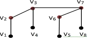
Figure 2. GraphB2
From Figure 2, we can easily see that γe −set S of Bn is {v2, v3}. Actually, these vertices are root vertices ofB2.
From Figure 3, we can easily see that B3 includes two subgraphs B2. We assume that γe −set S0 of B3 is formed by the minimum exponential dominating set of B2. That is, the root vertices of each subgraph B2 are in S. Hence, S0 = {v2, v3, v6, v7} and
wS0(v) ≥ 1 for all vertices of B3. But, in this case S0 is not minimum set. Since the
vertices v3, v7 ∈ S are adjacent, we must remove any one from the S. Hence, we have
γe(B3) = 2(γe(B2)−1) + 1 = 3.
Forn >3, in a similar manner, the minimum exponential domination number ofBn is
γe(Bn) = 2(γe(Bn−1)−1) + 1. (1)
When we use this result in recursive formula which we have obtained for Bn, we have
γe(Bn) = 2i(γe(Bn−i)−1) + 1 for 1≤i≤n−2. We must prove this formula by induction
oni. Let∀n∈Z+ and n≥3.
Wheni= 1, we have γe(Bn) = 2(γe(Bn−1)−1) + 1 and it is true by (1). We assume that the result is true fori=kand prove it fori=k+ 1. By induction hypothesis and (1), we get
γe(Bn) = 2k(γe(Bn−k)−1) + 1
= 2k(2(γe(Bn−k−1)−1) + 1−1) + 1 = 2k(2(γe(Bn−k−1)−1)) + 1
= 2k+1(γe(Bn−k−1)−1) + 1.
That is, the formula is true fori=k+ 1. Hence, we have γe(Bn) = 2i(γe(Bn−i)−1) + 1
for 1≤i≤n−2. Initial conditionn= 2 is achieved fori=n−2. We obtain the following formula.
γe(Bn) = 2i(γe(Bn−i)−1) + 1
= 2n−2(γe(Bn−(n−2))−1) + 1 = 2n−2(γe(B2)−1) + 1 = 2n−2(2−1) + 1 = 2n−2+ 1.
The proof is completed.
Definition 3.2. [15] For integer t≥ 2 and r ≥1, the comet graph Ct,r is defined to be
the graph of ordert+r obtained from disjoint union of a starK1,t−1 and a pathPr with r
vertices by adding an edge joining the central vertex of the star with an end-vertex of the path.
Theorem 3.2. The exponential domination number of a comet graph is given byγe(Ct,r) =
γe(Pr+2) =d(r+ 3)/4e.
Proof. Comet graph Ct,r includes the subgraphs Pr+2 and K1,t−1. One of Pr+2 is center vertexc∈V(K1,t−1) and the other one is pendant vertex v ∈V(K1,t−1). We know that, there is only center vertex c in γe−set of K1,t−1 and γe(K1,t−1) = 1. Also, we know that by Theorem 2.1, the exponential domination number of Pr+2 is d(r+ 3)/4e. If one of the vertices ofγe−setof Ct,r isc∈V(K1,t−1), then all vertices ofK1,t−1 and Pr+2 are exponentially dominated. Hence, we have
γe(Ct,r) =d(r+ 3)/4e.
Definition 3.3. [16] The completek−ary treeHnk of depthnis the rooted tree in which all vertices at level n−1 or less have exactly k children, and all vertices at level n are leaves.
Theorem 3.3. The exponential domination number of a completek−arytreeHnkis given by γe(Hnk) =kn−1.
Proof. The graph Hnk has k children for every vertices except leaves. For example, the graphH2k is obtained by combining kgraphs H1k with a root vertex. Similarly, the graph
Hk
3 is obtained by combiningkgraphs H2k with a root vertex. If we continue in a similar manner, we can easily see that the graphHnkis obtained by combiningkgraphsHnk−1 with a root vertex. Hence, the graphHnk contains previous ki graphs Hnk−i for 1≤i≤n−1. Then, we have the following generalized formula.
Hnk = kHnk−1 = k(k(Hnk−2)) = k(k(k(Hnk−3)))
...
= ki(Hnk−i).
So, we obtain Hnk = ki(Hnk−i) for 1 ≤ i ≤ n−1. The proof of exponential domination number ofHnk is examined on the value n.
Figure 4. GraphH12
From Figure 4, we can easily see that γe−set S of H12 is{v1}. This vertex is also the root vertex.
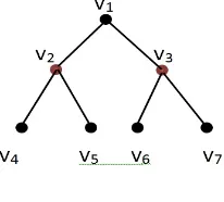
Figure 5. GraphH22
From Figure 5, we can easily see thatH22 includes two subgraphs H12. γe−set ofH22 is {v2, v3}. The vertices of this set are the vertices of γe−set of two H12. Hence, for n≥1 and 1≤i≤n−1
γe(Hnk) =kγe(Hnk−1). (2) When we use this result in recursive formula which obtained for Hnk, we have γe(Hnk) =
kiγe(Hnk−i) for n ≥ 1 and 1 ≤ i ≤ n−1. We must prove this formula by induction for
When i= 1, we have γe(Hnk) =k . γe(Hnk−1) and it is true by (2). We assume that the result is true fori= 5 and prove it fori=s+ 1. By induction hypothesis and (2), we get
γe(Hnk) = ksγe(Hnk−s)
= ks(kγe(Hnk−s−1)) = ks+1γe(Hnk−s−1).
That is, the formula is true fori=s+ 1. Hence, we haveγe(Hnk) =kiγe(Hnk−i) forn≥1
and 1≤i≤n−1. Initial conditionn= 1 is achieved for i=n−1. Hence, we obtain the following formula.
γe(Hnk) = kiγe(Hnk−i)
= kn−1γe(Hnk−(n−1)) = kn−1γe(H1k) = kn−1.
The proof is completed.
Definition 3.4. [17]
A tree T is called a caterpillar, if removal of all its pendant vertices results in a path called the spine of T , denoted by sp(T). If all vertices of sp(T) have equal number of pendant vertices, then the resulting graph is called a regular caterpillar. A regular caterpillar can also be defined as the corona of two special graph types. That is, ifTn,m is
a regular caterpillar, thenTn,m∼=Pn◦mK1.
Theorem 3.4. The exponential domination number of regular caterpillar Tn,m is given
by γe(Tn,m) =d(n+ 1)/2e.
Proof. Regular caterpillarTn,mhas vertices ofPn(or the spine) andmthe pendant vertices
that attached each vertex ofPn. LetSbeγe−setofTn,m. Assume that, we add all vertices
of Pn to S to dominate all pendant vertices. Hence, the condition wS(v) ≥ 1 satisfy for
all pendant vertices. But this set is not minimum exponential dominating set. Thus, S
must consist of the vertices with d(u, v) = 2 in < V(Tn,m)−(S− {u}) >, whereu ∈ S,
v∈V(Tn,m)−S. Ifd(u, v) = 2, we must add a vertexw inPn toS that this vertex is at
distance 2 fromu. Hence, the conditionwS(v) = 1 satisfy.
If n is odd, it is clear to see that the vertices which generate S are also the vertices of independent set of the spine graphPn. Hence, for every vertexxinV(Pn)−S,wS(x) = 1.
We haveγe(Tn,m) =dn/2e= (n+ 1)/2 =d(n+ 1)/2e.
If n is even, unlike the previous condition it is not enough to exponential dominate the last vertex vn of spine graph Pn with dn/2e vertices from the graph Pn. Because, the
weight of S at the vertex vn is 1/2. Hence, we must also add vn to S. Thus, we have
γe(Tn,m) =dn/2e+ 1 =n/2 + 1 =n/2 + 2 =d(n+ 1)/2e.
Whethern is odd or even, combining two cases we have,γe(Tn,m) =d(n+ 1)/2e.
The proof is completed.
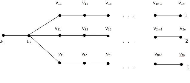
Figure 6. Tree Ent
Theorem 3.5. The exponential domination number of tree Ent is given by
γe(Ent) =
dn+ 1/4et, if t≤2n
, n≡2 (mod 4) dn+ 1/4e2n, if t >2n
bn+ 1/4ct+ 1, if t <2d(u1,v)
bn+ 1/4ct, if 2d(u1,v) ≤t <2n+d(u2,v)−1 , n≡0,1,3 (mod 4) bn+ 1/4c2n+d(u2,v)−1, if t≥2n+d(u2,v)−1
where,
d(u1, v) =
3, if n≡3 (mod 4) 4, if n≡0 (mod 4) 5, if n≡1 (mod 4)
and,
d(u2, v) =d(u1, v)−1,
where u1, u2 vertices not in legs of Ent and v is vertex of legs.
Proof. Let S be γe−set of Ent. For the vertex vin (1≤i≤t) on all legs, deg(vin) = 1.
The vertex vin−1of some legs must be added to S to exponentially dominate the vertex
vin. Each leg has the path graph Pn. The proof can be proved as the proof of Theorem
2.1. We start constructing S starting with the vertex vin−1 (i= 1) on the first leg and take each vertex at distance 4 from selecting vertex on the leg. Hence, we addd(n+ 1)/4e vertices to S from the first leg inEnt. We use similar argument for other legs. Thus, we have four cases depending on|V(Pn)|in the graph Ent.
For n ≡ 0,1,3 (mod 4), we get same results. Therefore we examine the proof into two cases.
Case 1: Letn≡2 (mod 4).
IfSis constructed as described above for any leg ofEnt, then we getS={vin−1, ..., vi5, vi1}. Similar argument is not applied for each leg in Ent. Because, this approach is contradict with the definition of the minimum exponential dominating set.
toS. Therefore, the vertices of S should be taken from a certain number of legs in Ent. So, every vertex ofV(Et
n)−S is exponentially dominated by S. This value depends on
the distance between vertices of different legs.
Letvinandvj1be the vertices of theithandjthlegs, respectively, wherei, j∈ {1,2, ..., t}, i6=
j. Note that d(vj1, vin) =n−1 +d(u2, vj1) + 1. Since,d(u2, vj1) = 1, we getd(vj1, vin) =
n+ 1. Hence, we have two subcases depending on the number of legs inEnt.
Subcase 1.1. If t < 2d(vj1,vin)−1, that is t < 2n then the vertices of S should be taken from each leg. Hence, we have ws(z) ≥ 1 for every z in V(Ent). So, we obtain
|S|=d(n+ 1)/4et.
Subcase 1.2. If t ≥ 2n, then the vertices of S should be taken from only 2n legs. Hence, we get|S|=d(n+ 1)/4e2n.
Case 2: Letn≡0,1,3 (mod 4).
IfS is constructed as in Case 1, then we get three differentS sets depending onnmod 4. These set are
S={vin−1, ..., vi7, vi3}orS ={vin−1, ..., vi8, vi4} orS ={vin−1, ..., vi6, vi2}.
Hence, we must get b(n+ 1)/4c vertices to S from only one leg in Ent. The minimum distance between u1 ∈ V(Ent) and vi2 ∈ S or vi3 ∈ S or vi4 ∈ S is d(u1, vi2) = 3,
d(u1, vi3) = 4 andd(u1, vi4) = 5. The rest of the proof is performed as in Case1.
Note that,d(vin, vj2) =n−1+d(u2, vj2)+1,d(vin, vj3) =n−1+d(u2, vj3)+1,d(vin, vj4) =
n−1 +d(u2, vj4) + 1.
We denote the vertices vj2, vj3 and vj4 by v to give a generalized formula. So, we have three subcases depending on the number of legs.
Subcase 2.1. If t <2d(u1,v), then the vertices of S should be taken from each leg. In this case, wS(u1) ≥ 1 for u1, u2 ∈ V(Ent) and the condition wS(u2) ≥1 is not satisfied. Hence, we must add the vertexu1 oru2 toS. Therefore, we get |S|=b(n+ 1)/4ct+ 1.
Subcase 2.2. If 2d(u1,v)≤t≤2n+d(u2,v)−1 then the vertices ofS should be taken from each leg. Thus,wS(z)≥1 satisfies for everyz inV(Ent). We obtain|S|=b(n+ 1)/4ct.
Subcase 2.3. Ift ≥2n+d(u2,v)−1, then the proof is similar to Subcase 1.2. Hence, we get|S|=b(n+ 1)/4c2n+d(u2,v)−1.
Summing Case 1 and Case 2, we obtain exponential domination number ofEnt.
The proof is completed.
4. Conclusion
The vulnerability of a communication can be measured by the exponential domina-tion number of the graph describing the network. The exponential dominadomina-tion number has been studied as a vulnerability parameter introduced in [16]. Calculation of the ex-ponential domination number for simple graph is important because if one can break a more complex network into smaller networks, then under some conditions the solutions for the optimization problem on the smaller networks can be combined to a solution for the optimization problem on the larger network.
References
[1] Anderson, M., Brigham, R. C., Carrington, J. R., Vitray, R. P., Yellen, J., (2009). On Exponential Domination ofCmxCn, AKCE J.Graphs. Combin.,6, No. 3 341-351.
[2] Ayta¸c, V. and Turacı, T., (2017). Exponential Domination and Bondage Numbers in Some Graceful Cyclic Structure, Nonlinear Dynamics and Systems Theory, 17(2), 139-149.
[4] Ayta¸c, A., Odaba¸s, Z. N. and Turacı, T., (2011). The bondage number of some graphs, Comptes Rendus de Lacademie Bulgare des Sciences, vol. 64, no. 7, pp. 925930.
[5] Ayta¸c, A., Turacı, T. and Odaba¸s, Z. N., (2013). On the bondage number of middle graphs, Mathe-matical Notes, vol. 93, no. 5-6, 795 801.
[6] Ayta¸c, A. and Odaba¸s, Z. N., (2011). Residual Closeness of Wheels and Related Networks, Int. J. Found. Comput. Sci., 22, pp. 12291240.
[7] Ayta¸c, A. and Berberler, Z. N., (2017). Binding Number and Wheel Related Graphs, Int. J. Found. Comput. Sci., 28(1), pp. 29-38.
[8] Ayta¸c, A. and Berberler, Z. N.,(2017). Robustness of regular caterpillars, Int. J. Found. Comput. Sci., accepted.
[9] Ayta¸c, A. and Odaba¸s Berberler, Z. N. Network robustness and residual closeness, RAIRO Operations Research, DOI: https://doi.org/10.1051/ro/2016071, appear.
[10] Ayta¸c, A. and Odaba¸s, Z. N., (2010). Computing the rupture degree in composite graphs, Int. J.Found. Comput. Sci., 21(03), pp. 311-319.
[11] Ayta¸c, A. and Odaba¸s, Z. N., (2009). On Computing The Vulnerability Of Some Graphs As Average, International Journal of Pure and Applied Mathematics, 55(1), pp. 137-146.
[12] Berberler, M. E and Berberler, Z. N., (2017). Measuring the vulnerability in networks: a heuristic approach, ARS COMBINATORIA, accepted.
[13] Chartrand, G. and Lesniak, L., (1986). Graphs and Digraphs, Second Edition, Wadsworth. Monterey. [14] Cormen, T., Leiserson, C. E. and Rivest, R. L., (1990). Introduction to Algorithms, The MIT Pres.
(Fourth edition).
[15] Cymen, M., Pilipczuk, M. and Skrekovski, R., (2010). Relation between Randic index and average distance of trees, Institute of Mathematics, Physics and Mechanics Jadranska, 48, Slovenia, 1130p. [16] Dankelmann, P., Day, D., Erwin, D., Mukwembi, S., Swart, H., (2009). Domination with exponential
decay, Discrete Mathematics 309, pp. 5877-5883.
[17] Gallian J. A., (2008). A dynamic survey of graph labeling, Elect. Jour. Combin. 15, DS6. [18] Hartsfield, N. and Ringel, Gerhard., (1990). Pearls in Graph Theory, Academic Press, INC.
[19] Frucht, R. and Harary, F., (1970). On the corona two graphs, Aequationes Math., vol.4, pp. 322-325. [20] Haynes, T. W., Hedetniemi, S. T. and Slater, P. j. Fundamentals of Domination in Graphs, Marcel
Dekker,Inc., New York.
[21] Haynes, T. W., Henning, M. A., Van Der Merwe, L.C., (2007). The complementary product of two graphs, Bull. Instit. Combin. Appl. 51, pp. 21-30.
[22] Haynes, T. W., Henning, M. A., Van Der Merwe, L. C., (2009). Domination and Total Domination in Complementary Prisms, J. Comb. Optim 18, pp. 23-37.
[23] Hedetniemi, S. T. and Laskar, R. C., (1990). Bibliography on domination in graphs and some basic definitions of domination parameters, Discrete Mathematics, vol. 86, no. 1-3, pp. 257-277.
[24] Odaba¸s, Z. N. and Ayta¸c, A., (2013). Residual closeness in cycles and related networks, Fundamenta Informaticae 124 (3), pp. 297-307.
[25] Odaba¸s, Z.N. and Ayta¸c, A., (2012). Rupture Degree and Middle Graphs, Comptes Rendus De L Academie Bulgare Des Sciences 65(3), pp. 315-322.
[26] Turacı, T. and Ayta¸c, V. Residual closeness of splitting networks, Ars Combinatoria ( accepted). [27] West, D. B., (2001). Introduction to Graph Theory (Second edition).