ABOUT AN ALGORITHM OF FUNCTION APPROXIMATION BY THE LINEAR SPLINES
B.BAYRAKTAR1, V.KUDAEV2,§
Abstract. The actual application for the problem of best approximation of grid func-tion by linear splines was formulated. A mathematical model and a method for its solution were developed. Complexity of the problem was that it was multi - extremal and could not be solved analytically. The method was developed in order to solve the problem of dynamic programming scheme, which was extended by us. Given the appli-cation of the method to the problem of flow control in the pressure-regulating systems, the pipeline network for transport of substances (pipelines of water, oil, gas, and etc.) that minimizes the amount of substance reservoirs and reduces the discharge of sub-stance from the system. The method and the algorithm developed here may be used in computational mathematics, optimal control and regulation system, and regressive analysis.
Keywords: grid functions, the best approximation, minimal deviation, linear splines, dynamic programming, optimal regulation.
AMS Subject Classification: 65D15, 49L20, 49J35
1. Introduction
As it is known functions may be approximated with linear splines. It is one of the main directions in computational mathematics and has a number of applications in systems and process modeling.
Problems of asymptotically optimal nodes where splines may be coupled with selection and determine the order of the best spline approximations with increasing number of nodes are solved for different kinds of splines [1-4]. Optimal nodes selection not only decreases approximation error but also allows making qualitative conclusions on behavior in modeling process. For instance, it helps to determine the transition point in researches of transitional process. However, until now, algorithms of optimal choice of gluing unit splines have not been developed.
Linear splines are used in systems of robotized design, optimal control and regulation in systems, and statistics [5, 6]. But there is no algorithm for optimal nodes selection to glue splines together though it is the simplest kind of splines. The algorithm to choose optimal nodes for interpolation type problem, i.e., the case when nodes of linear spline coupling are set in grid function diagram, is represented in the article [7]. The method
1
Uludag University, Education Faculty, Gorukle Campus, Bursa, Turkey. e-mail: [email protected];
2
Institute of Computer Science and Problems of Regional Management of Kabardino-Balkar Scientific Centre of RAS, Russia.
e-mail: [email protected];
§ Manuscript received: February 07, 2016; accepted: May 05, 2016.
TWMS Journal of Applied and Engineering Mathematics, V.6, No.2; cI¸sık University, Department of Mathematics, 2016; all rights reserved.
of solution to the problem of the best approximation for grid function with linear splines with minimal deviation is presented in our article.
2. Formulation of the problem
The problem. Let us give the discrete set T ={ti∈R |ti < ti+1, i= 0,1,2, ..., n−1}
and functionf:T → R. It requires function f(t) approximate by piecewise liner function
lm (t, x0, y0, ..., xm, ym) with a given number of lines segments m ≤ n, where xk∈ T, yk∈R, for k=0,1, ..., mdesired coordinates of its nodes, t0=x0 < ... < xm=tn, so that the deviationlm from f must be minimal:
ρ(ti, x0, y0, ..., xm, ym) = max
0≤i≤n|f(ti)−lm(ti, x0, y0, ..., xm, ym)| →min (1)
Let us prove the existence of the decision (1).
There is finite number of sets (x0, x1, ..., xm) as the scale t is discrete and ∀i∈(0,m),
∃k∈(0,n),xi=tk. Let ( ˆx0,xˆ1, ...,xˆm) be any among any sets, and ˆρis deviationlm fromf
for the set, for instance, ˆy0=f( ˆx0), ˆy1=f( ˆx1),..., ˆym=f( ˆxm). Then it is evident, at optimal
decision of the problem (1), if it is exist,ρopt≤ρˆ. Thus, the problem (1) is equivalent to
this one:
(
ρ= max0≤i≤n|f(ti)−lm(ti, x0, y0, ..., xm, ym)| →min
ρ≤ρˆ (2)
Now let (ˆx0,xˆ1, ...,xˆmˆ) be an arbitrary fixed set. Multiplicity of values y0, y1, ..., ym
that satisfies
f(ˆxj)−ρˆ≤yj ≤f(ˆxj) + ˆρ, j= 0,1, ..., m (3)
is limited and covered as it represents m dimensional cube, and the function (1) is con-tinuous in it. That is why the problem (2) on this set has the decision or its multiple solutions are empty. Having enumerated all the possible sets (x0, x1, ..., xm) and having
compared decisions on those among them where multiplicity of decisions is not empty, we will find optimal decision for initial problem.
3. The problem solution algorithm
We will now give definitions of some terms and concepts that are used in the article.
Definition 3.1. Vertical or layer is called an ordered set of numbers of possible discrete values of the function at a given point.
Definition 3.2. The smallest possible deviation of a given function from a straight line is called the potential or an error.
Definition 3.3. An arc is called an ordered pair of numbers of vertices, respectively, from the previous and subsequent layers, the relationship between which is possible.
The solution of the problem consists of two phases in each of which the constructed expanded scheme of the Dynamic Programming (DP) is used in a special way. In contrast to the standard scheme DP in the proposed scheme, the intersection of points on the verticals is not empty.
At the first phase we solve the problem of the best interpolation of the given function. This decision is made for the initial solution of a problem of approximation. At the second stage, verticals are built in the received optimum interpolation points and the problem of the best approximation of function is solved.
3.1. Algorithm of the solution of a problem of interpolation. For convenience, we introduce the following notation:
y(t) – straight line equation passing through two given points (i, f(i)) and (q, f(q)); δiq – maximum deviation of a line segment connecting the points with coordinates (i, f(i))
and (q, f(q)) from a given function, wherei= 0,1,2, ..., n−1,q=i+ 1, i+ 2, ..., n; Pqj – potential q vertex j layer, where j= 1,2, ..., m, q=i+ 1, i+ 2, ..., n;
Gjq– discrete set of vertices of the previous (j−1) layer incident to q vertex of j layer;
Then,
y(t) = (t−i)f(q)−(t−q)f(i)
i−q (4)
δiq = max ∀t∈[xi,xq]
|f(t)−y(t)| (5)
Then Bellman-Dijkstras recurrent process [8] for points potentials calculation in layers occurs:
Pqj+1 = min
i∈Gjq
max{Pij, δiq}, q= 0,1,2, ..., m−1 (6)
1. We set the number of linear splines -m.
2. For alliandq let us calculate errorsδiq forming a triangular Matrix of Errors (ME) of
interpolation:
δ01 δ02 δ03 δ04 ... δ0n δ12 δ13 δ14 ... δ1n ... ... ... δn−2,n−1 δn−2,n
δn−1,n
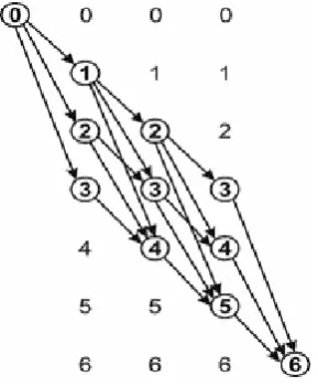
3. Using this matrix we develop the scheme DP.
3.1 For this purpose in the 1st layer of the scheme, all elements are marked all elements (that are led round by circle, see figure 1) accessible from the zero vertex, that is vertex corresponding to the 1st line ME. In the 2nd layer, all those vertices are placed, which are reachable at least from one marked vertex of the first layer and so on. In the last layer, all those vertices are placed, which are reachable from the marked vertices of a penultimate layer and also those vertices from which the last vertexN is achievable.
3.2 Affixing corresponding weights (errors) to the arcs connecting the vertices of adjacent layers.
4. Potential of zeros vertex, apparently, is equal to zero.
5. We count potentials of the subsequent layer on the basis of the potentials of vertices of the previous layer and errors corresponding to the arches connecting the previous and subsequent layers on formula (6). The arc corresponding to value Ppj+1 is remembered.
Calculations of potentials proceed until we reach the last, m layer with n vertex.
6. After that we move from the last vertex by the beginning the column DP on the allocated arcs, remembering the vertices corresponding to them. The sequence of these vertices also give the best interpolation of the given function to the linear splines with a minimum potential ˆδ=Pnm−1.
3.2. Algorithm of the solution to a problem of approximation. We take result of the solution to a problem of the best interpolation for the initial solution to a problem of approximation. To solve this problem, we do not need to build a matrix of error. Formation of the best path from the starting point to the end was made sequentially, starting with the first layer, then the second, etc. up to and including the last layer.
Let us enter the following designations: k– predetermined positive integer;
s– integer, ands=−k, ...,−1,0,1, ...,+k; j – number of a layer and j= 0,1, ..., m−1; ˆ
δ – interpolation error;
f(xj+sδˆ) =fsj; for examplef(x3)−2ˆδ=f−32
(xj, fsj) – coordinates of points which numbers form verticals of each of mof layers of the
scheme DP;
yjis(t)– equation of a line segment connecting the i–th point of j-th layer and s–th point (j+ 1)–th layer;
δjis –maximum deviation of a straight line segmentyisj(t) from a function graph f(t) on a piece [xj, xj+1].
Psj – potential of s–th point, that is, the point (xj, fsj) ofj –th layer.
Then
yisj(t) = f
j+1
s −fij xj+1−xj
t−f
j+1
i xj−f j sxj+1 xj+1−xj
(7)
δjis= max ∀t∈[xj,xj+1]
|f(t)−yjis(t)| (8)
Potential of i– th point of (j+ 1) –th layer, that is, the point (xi, fij+1), will be Pij+1 = min
−k≤s≤kmax{P j
s, δis} (9)
1. We take the best solution to a problem of interpolation for the initial decision: x0 →x1→...→xm→xn with a margin error ˆδ;
2. We form scheme DP layers which each layer contains points (xi, fsi).
3. Sequentially we calculate potentials of vertices of layers.
3.1 Potential of vertices of the 1st layer – are valuesδsi0– that is, evasion of straight lines connecting a pointx0 with vertices of the 1st layer (s, i=−k, ...,+k).
3.2 Let all the potentials be already calculatedPsj, vertices ofj– th layer (s=−k, ...,+k).
of the previous layer proceeding from, which potentiali–th vertex of (j+ 1)–th layer was received.
4. In the last layer we choose vertex with a minimum potential p = min∀s{Psm}, which
gives the optimum path from the last layer into the first layer. On this trajectory nodes define the best approximation of a given function.
4. Results of numerical experiment of the problems of interpolation and approximation of function
The developed algorithms are realized in programming language C++ in the environ-ment of Builder 6.0. On the example of periodic function off(x) =sinx on an interval [0,2π] numerical experiments of interpolation and approximation for n= 72 and m= 13 are made. Results of numerical experiment are presented on screen forms (Fig. 2 and 3) and are summarized in Table 1-3.
Fig. 2. Screen shot for optimal interpolation
Displayed results: n=73, layers quantity m=13, lines quantity-12, minimal deviation δˆ= 0.02230.
Table 1. Optimal coordinates of the interpolation
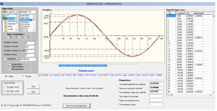
Fig. 3. Screen shot for optimal approximation
Displayed results: n=73, layers quantitym=13, lines quantity-12, initial valueδˆ= 0.02230, minimal deviation 0.01391.
Table 2. Optimal coordinates of the approximation for k= 5
N α(deg) sin(α) xj N α(deg) sin(α) xj 1 0 0.0000 0.0000 8 220 -0.6428 -0.6473 2 40 0.6428 0.6562 9 245 -0.9063 -0.9152 3 65 0.9063 0.9152 10 270 -1.0000 -1.0089 4 90 1.0000 1.0089 11 295 -0.9063 -0.9152 5 115 0.9063 0.9152 12 320 -0.6428 -0.6562 6 140 0.6428 0.6473 13 360 0.0000 0.0000 7 180 0.0000 0.0134
Table 3. Results of approximation at various quantities of points on
ver-ticals (here ˆδ= 0.02230 and received from interpolation)
Quantity points on Computing the verticals(2k+1) δopt Time(sec)
3 0.02228 0
5 0.01503 0
7 0.01487 0
9 0.01503 0
11 0.01391 1
13 0.01487 1
15 0.01423 1
5. Optimization of the flow control in the pressure-regulating system
of substance moving in system from the tank, and surplus giving from pump station -surplus arrival in the tank.
One needs to minimize the volume of the reservoir for a given number of switching pump stations and substance consumption schedule. When the optimal solution of the problem is reached, the amount of substance that consumers receive hourly is very close to the required level.
In the article [9] the problem was solved by local variations method and the solution was specified in the vicinity of the locally optimal trajectory. The method provided in the article [10] is in the following. The descent to the optimum is carried out simultaneously from several initial solutions built by direct search on the rough grid. Then construct an iterative process whereby ”narrowing of neighborhoods” is clarified, each of these solutions with the prescribed accuracy. Among these solutions, the best solution is chosen. The method is effective in a small number of segments.
Let g =g(t) be a discrete step-function of time the setting consumption of amount of substance by system in each hour days percentage of total of substance, then accumulation of substance in the tank can be expressed by integral function:
f(t) =R0tg(x)dx, wheret= 1,2,3, ...,24.
For the solution of a problem of minimization of volumes of tanks it is required to approximate integral function of f(t) the given quantity of the linear splines the least evading from functionf(t) and to construct a step-function. This step-function will also be the schedule of work of the pump station.
The method provided here allows us to solve the problem with accuracy (defect) δ without restrictions on number of branches.
The screenshot (Fig. 4) and Table 5 provide information for management manager of the pipeline system. There is a recommendation for (optimal) 5-mode schedule pumping station (thin line) and a maximum of 24-hour substance supply schedule (bold line) in its center:
In the table of graph to the right: Consumption by an hour a day (percentage of total consumption ), Stock change by an hour a day, Stock ++ –total accumulation. The minimum volume of the regulatory1.08368% from the total consumption.
Table 4. Information of control system for pipeline system manager
The period of time (h) 0–3 3–5 5–8 8–14 14–21 21–24 Delivery for network(%) 2.47682 3.50000 5.05238 4.16667 5.01211 3.49000
6. Conclusion
We formulated the actual for application a mathematical model of the problem of best approximation of the grid functions by linear splines and the method of its solution.
To solve the problem, we developed a method based on the idea of the DP method. The expanded scheme DP, which differed from the reference scheme DP in that the point set on verticals could not be empty, was offered.
The problem was solved in two stages: At the first stage, the problem of the best interpolation of function was solved. At the second stage, the problem of the best approx-imation was solved. The problem of approxapprox-imation for the initial solution to the problem was taken as a base for the solution to the interpolation problem.
The application was implemented to the problem of control optimization of flows in the pressure-regulating systems, supply and consumption of substances.
7. Acknowledgment
Researched with the support of Russian Fond of Basic Researches grants 13-01-00929-a, 13-07-01002-a, 15-01-05844-a which is gratefully acknowledged.
References
[1] Boor,K., (1985), A practical guide to splines, Radio and Communication.
[2] Grebennikov,A.I., (1976), The choice of nodes in the spline approximation of functions., Zhurnal Vychislitel’noi Matematiki i Matematicheskoi Fiziki, 16 (1), pp. 219-223.
[3] Ligun,A.A. and Shumeiko,A.A., (1997), Asymptotic methods for rebuilding curves, Institut Matem-atici NAN Ukrainy, Kiev.
[4] Walters,H.J., (2004), A Newton-type method for computing best segment approximations, Commu-nications on Pure and Applied Analysis, 3 (1), pp. 133-149.
[5] Shumeiko,A.A. and Shumeiko,E.A., (2011), On the construction of asymptotically optimal piecewise-linear regression, Informatics and Mathematical Methods in Simulation, 1 (2), pp. 99-106.
[6] Thamaratnam,K., Claeskens,G., Croux,C. and Salibian-Barrera,M., (2010), S-estimation for penalised regression splines, Journal of Computational and Graphical Statistics, 19 (5), pp. 609-625.
[7] Pakhnoutov,I.A., (2011), Vybor uzlov sglazhivaniya lineynymi splaynami, Izvestia Kaliningradskogo Tekhnicheskogo Universiteta, 23, pp. 122-126,
[8] Christofides,N., (1978), Graph theory. An algorithmic approach, Mir, Moskva.
[9] Kudaev,V.C. and Bayraktarov,B.R., (2013), Regulation optimization in network systems., News of Kabardin-Balkar Scientific Center of Russian Academy of Sciences, 6 (56), pp. 33-38.
Bahtiyar BAYRAKTAR graduated from the Faculty of Mathematics of Kabardino - Balkarian State University (USSR) in 1976. From 1977 to 1989 he worked in the Scientic Research Institute of Applied Mathematics and Mechan-ics(Nalchik, Russia). In 1992 he got his Ph.D. degree from Rostov State University. His research areas are calculus of variations and optimal control. He is an Assistant of Prof. of Pedagogical Faculty of Uludag University in Turkey.