ISSN: 2008-6822 (electronic)
http://dx.doi.org/10.22075/ijnaa.2015.270
An assessment of a semi analytical AG method for
solving two-dimension nonlinear viscous flow
S. Tahernejad ledari, H. Mirgolbabaee, D. Domiri Ganji∗
Department of Mechanical Engineering, Babol University of Technology,P.O. Box 484, Babol, Iran
(Communicated by R. Memarbashi)
Abstract
In this investigation, attempts have been made to solve two-dimension nonlinear viscous flow between slowly expanding or contracting walls with weak permeability by utilizing a semi analytical Akbari Ganji’s Method (AGM). As regard to previous papers, solving of nonlinear equations is difficult and the results are not accurate. This new approach is emerged after comparing the achieved solutions with Numerical method and exact solution. Based on the comparison between AGM and numerical methods, AGM can be successfully applied for a broad range of nonlinear equations. Results illustrate, this method is efficient and has enough accuracy in comparison with other semi analytical and numerical methods. Ruge-Kutta numerical method, Variational Iteration Method (VIM), Homotopy Perturbation Method (HPM) and Adomian Decomposition Method (ADM) have been applied to make this comparison. Moreover results demonstrate that AGM could be applicable through other methods in nonlinear problems with high nonlinearity. Furthermore convergence problems for solving nonlinear equations by using AGM appear small.
Keywords: Adomian Decomposition Method (ADM); Akbari-Ganji Method (AGM); Homotopy Perturbation Method (HPM); Variational Iteration Method (VIM).
2010 MSC: Primary 00A72; Secondary 37A60.
1. Introduction
The flow of Newtonian and non-Newtonian fluids in a porous surface channel has attracted the interest of many investigators in view of its applications in engineering practice, particularly in industries. Examples of these are the cases of boundary layer control, transpiration cooling and
∗Corresponding author
Email address: [email protected](D. Domiri Ganji)
gaseous diffusion. Theoretical research on steady flow of this type was initiated by Berman [1] who found a series solution for the two-dimensional laminar flow of a viscous incompressible fluid in a parallel-walled channel for the case of a very low cross-flow Reynolds number. After his work, this problem has been studied by many researchers considering various variations in the problem, e.g., Choi et al. [2] and references cited therein. For the case of a converging or diverging channel with a permeable wall, if the Reynolds number is large and if there is suction or injection at the walls whose magnitude is inversely proportional to the distance along the wall from the origin of the channel, a solution for laminar boundary layer equations can be obtained [3].
Most scientific problems such as two-dimensional viscous flow between slowly expanding or con-tracting walls with weak permeability and other fluid mechanic problems are inherently nonlinear. Except a limited number of these problems, most of them don’t have analytical solution. There-fore, these nonlinear equations should be solved using other methods. In the analytical perturbation method, we should exert the small parameter in the equation. Therefore, finding the small parameter and exerting it into the equation are difficulties of this method. Since there are some limitations with the common perturbation method, and also because the basis of the common perturbation method is upon the existence of a small parameter, developing the method for different applications is very difficult. Therefore, many different methods have recently introduced some ways to eliminate the small parameter. In this study we are comparing the efficiency and accuracy of some of these methods with Akbari-Ganji’s Method [4, 5, 6].
The Homotopy perturbation method (HPM) [7, 8, 9] is well-known method to solve the nonlinear equations. This method is introduced by He [10, 11] for the first time. This method has been used by many authors such as Ganji in [12, 13] and the references therein to handle a wide variety of scientific and engineering applications such as linear and nonlinear, homogeneous and inhomogeneous as well, because these methods continuously deform a difficult problem into a simple one, which is easy to solve.
The other method which could be mentioned is variational Iteration Method (VIM) [14, 15, 16] by J.H.He, this method also has been used by many scientists and recently some parts of it has been developed because of introducing some new methods for identification of the Lagrangian multiplier which is used in VIM formula [17].
And the last method which has compare to AGM in this paper is Adomian Decomposition Method (ADM) [18, 19, 20], At the beginning of the 80s, a new method later called ADM for solving various kinds of nonlinear equations had been proposed by Adomian [21, 22]. The convergence of Adomian’s method has been investigated by several authors K. Abbaoui, Y. Cherruault [23, 24]).
Description Symbol
Homotopy Perturbation Method HPM
Variational Iteration Method VIM
Adomian Decomposition Method ADM
Akbari Ganji’s Method AGM
Velocity component in x direction bu
Velocity component in y direction bv
Dimensionless pressure bp
Non-dimensional wall dilation rate which is dened positive for expansion α
Permeation Reynolds number which is considered positive for injection Re
Axial coordinate bx
Axial coordinate yb
Time t
Kinematic viscosity ν
Density ρ
2. Mathematical Fourmulation
Consider the laminar, isothermal, and incompressible flow in a rectangular domain bounded by two permeable surfaces that enable the fluid to enter or exit during successive expansions or contractions [25]. One side of the cross section, representing the distance (2a) between the walls is taken to be smaller than the other two (W and L). Both walls are assumed to have equal permeability and to expand uniformly at a time dependent rate a. Furthermore, the origin x = 0 is assumed to be the center of the classic squeeze film problem. This enables us to assume flow symmetry about x = 0 . Under these assumptions, the equations for continuity and motion become:
∂bu ∂bx+
∂bv
∂yb (2.1)
∂bu
∂t +ub·( ∂bu ∂bx) +bv·
∂bv ∂yb= (
−1
ρ )·( ∂pb
∂bx) +v∇ 2
b
u (2.2)
∂bv
∂t +ub·( ∂bv ∂xb) +bv·
∂vb ∂yb= (
−1
ρ )·( ∂pb
∂by) +v∇ 2
b
v (2.3)
Where pb,ρ,ν and t are the dimensional pressure, density, kinematic viscosity, and time. Auxiliary conditions can be specified such as:
b
u(x,b 0) = 0,bv(a) = −bv(w) =−a
c (2.4)
∂bu
∂yb(x,b 0) = 0,bv(0) = 0,bu(0,yb) = 0 (2.5)
After some modification and special variable [10] and then we have:
d4
dx4F(x) +α
y d 3
dx3F(x) + 3
d2 dx2F(x)
+Re
d dxF(x)
d3 dx3F(x)
−Re
d dxF(x)
d2
dx2F(x) = 0
With the boundary conditions:
F(0) = 0, F(1) = 1, F0(1) = 0, F00(0) = 0 (2.7)
Where a prime denotes differentiation with respect to y: Note that Bermans [1] well-known ODE can be viewed as a special case of Eq. (2.6) with α = 0, so the above equation could be rewrite as follow:
d4
dx4F (x) +Re
d3
dx3F(x)
F (x)−
d dxF (x)
d2
dx2F (x)
= 0 (2.8)
3. Analysis of He’s Homotopy Perturbation Method
To illustrate the basic ideas of this method, we consider the following equation:
A(u)−f(r) = 0, r ∈Ω (3.1)
With the boundary condition of:
B(u,∂u
∂n) = 0, r∈Γ (3.2)
Where A is general differential operator, B a boundary operator, f(r) a known analytical function and Γ is the boundary of the domain Ω .Acan be divided into two parts, which are Land N, where
L is linear andN is nonlinear. Eq. (3.1) can therefore be rewritten as follows:
L(u) +N(u)−f(r) = 0, r ∈Ω (3.3)
Homotopy perturbation structure is shown as follows:
L(v)−L(u0) +p·L(u0) +p·[N(v)−f(r)] (3.4)
Or:
H(v, p) = (1−p)[L(v)−L(u0)] +p[A(v)−f(r)] = 0 (3.5)
Where:
v(r, p) : Ω×[0,1]→R (3.6)
In Eq. (3.4) or Eq. (3.5),p∈[0.1] is an embedding parameter and u0 is the first approximation that
satisfies the boundary condition. We can assume that the solution of Eq. (3.1) can be written as a power series inp, as following:
v =v0+p·v1+p2 ·v2+. . .= n
X
i=0
pi·vi (3.7)
And the best approximation for solution is:
u= lim
3.1. The Application of HPM
In this section, we will apply the HPM to nonlinear ordinary differential Eq. (2.8) with a boundary condition Eq. (2.7). According to the HPM, we can construct homotopy of Eq. (2.8) as follows:
H(x, p) = (1−p) d
4
dx4F(x)
+p
d4
dx4F (x) +R
d3
dx3F (x)
F (x)−
d dxF(x)
d2
dx2F(x)
(3.9)
We considerF(x) as follows:
F(x) = F0(x) +pF1(x) +p2F2(x) (3.10)
From Eq. (3.7), if the three terms approximations are sufficient, we will obtain with substituting u from Eq. (3.10) into Eq. (3.9) and some simplification and rearranging based on powers of p-terms, we have :
p0 : d
4
dx4F0(x) = 0 F0(0) = 0, F0(1) = 1, F
0
0(1) = 0, F
00
0(0) = 0
(3.11)
p1 :
d3
dx3F0(x)
F0(x)R−
d
dxF0(x)
d2
dx2F0(x)
R+ d
4
dx4F1(x)
F1(0) = 0, F1(1) = 0, F
0
1(1) = 0, F
00
1(0) = 0
(3.12)
p2 :
d3
dx3F0(x)
F1(x)R+
d3
dx3F1(x)
F0(x)R
−
d
dxF0(x)
d2
dx2F1(x)
R−
d
dxF1(x)
d2
dx2F0(x)
R+ d
4
dx4F2(x)
F1(0) = 0, F1(1) = 0, F
0
1(1) = 0, F
00
1(0) = 0
(3.13)
Solving Eq.s (3.11), (3.12) and (3.13) with boundary conditions, we have:
F0(x) = −1
2 x
3+3
2x (3.14)
F1(x) = Rx7
280 − 3Rx3
280 +
Rx
140 (3.15)
F2(x) =
R2x11
92400−
R2x9
3360 +
3R2x7
19600 +
73R2x3
107800 −
703R2x
1293600 (3.16)
The solution of this equation, when p→1 , will be as follow:
F(x) =F0(x) +F1(x) +F2(x) (3.17)
With assumption of Re= 1, F(x) would be as follow:
4. Variational Iteration Method
To illustrate the basic idea of variational iteration method, we consider the following general nonlinear system:
Lu+N u=g(x) (4.1)
Where L is a linear operator, N nonlinear operator, g(x) a homogeneous term. According to the variational iteration method, we can construct the following iteration formulation:
un+1(t) = un(t) +
Z t
0
λ(Lun(τ) +N un(τ)−g(τ)) dτ (4.2)
Where λ is a general Lagrangian multiplier [26, 27], which can be identified optimally via the vari-ational theory [28, 29].The subscript n indicates the nth approximation and
e
un is considered as a
restricted vaeiation [30, 31] , i.e.,δuen = 0, where λ is general Lagrange multiplier. For calculating
Lagrange multiplier we are doing the following steps:
1. Linear part of differential equation is solved by Laplace method and will be put equal (−1)n (wheren is the highest order derivative of the linear part)
2. We assume zero the boundary conditions of the problem
3. Wherever the result of Laplace is obtained parametrically, we change the variable, for example, if the result of the Laplace obtained is x, we replace it with (−1)n(−x)
4.1. The application of Variational iteration method (VIM)
First we construct a correction functional which reads:
Fn+1(x) =Fn(x) +
Z x
0 λ( d
4
dx4Fn(τ) +R((
d3
dx3Fn(τ))Fn(τ)
−( d
dxFn(τ))
d2
dx2Fn(τ))) dτ
(4.3)
Linear part of Eq. (4.2) is solved by Laplace method and will be put equal (−1)n (according to above description):
s4L[F]−s3F(0)−s2D(F)(0)−s(D(2))(F)(0)
−(D(3))(F)(0) = (−1)n −→n= 4−→s4L[F] = 1 (4.4)
F =L−1[1
s4] = x3
6 (4.5)
x= (−1)n·(τ −x) (4.6)
Substituting Eq. (4.6) into Eq. (4.1), so the Lagrange multiplier can be obtaining in that form:
λ= 1/6 (τ−x)3 (4.7)
As a result, we obtain the following iteration formula:
Fn+1(x) =Fn(x) +
Z x
0
(τ−x)3
6 (
d4
dx4Fn(τ) +R((
d3
dx3Fn(τ))Fn(τ)
−( d
dxFn(τ))
d2
dx2Fn(τ))) dτ
Now we start with an arbitrary initial approximation that satisfies the initial condition:
F0(x) =−1/2x3+ 3/2x (4.9)
Using the above variational formula (4.1) for n = 0, substituting Eq. (4.6) into Eq. (4.1) and after some simplifications, we have:
F1(x) =−1/2x3+ 3/2x+ Rx7
280 (4.10)
F2(x) =−1/2x3+ 3/2x+ Rx7
280 +
R3x15
30576000 +
R2x11
92400 −
x9R2
3360 (4.11)
In the same way, the rest of the components of the iteration formula can be obtained. With assump-tion of Re= 1, F(x) would be as follow:
F(x)∼=−0.5x3+ 1.5x+ 0.0035x7+ 0.00000003x15−0.00029x9
+0.0000108x11 (4.12)
5. Basic Idea of Adomian’s Decomposition Method
We consider a general nonlinear equation in the form:
Lu+R(u) +F(u) =g (5.1)
Where L is the operator of the highest-ordered derivatives which is assumed to be easily invertible,
Rthe linear differential operator of less order than L,F(u) presents the nonlinear terms andg is the source term. Thus we get:
Lu=g−R(u)−F(u) (5.2)
The inverseL−1 is assumed to be an integral operator, by applying the inverse operator L−1 to the
both sides of Eq. (40), we obtain:
u=f0+L−1(g−R(u)−f(u)) (5.3)
Where f0 is the solution of homogeneous equation:
Lu= 0 (5.4)
Involving the constants of integration. The integration constants involved in the solution of homo-geneous equation (5.4) are to be determined by the initial or boundary condition, since the problem is an initial value or a boundary value problem. The ADM assumes that the unknown function u(x) can be expressed by an infinite series of the form:
u(x) = ∞
X
n=0
un(x) (5.5)
And the nonlinear operatorF(u) can be decomposed by an infinite series of polynomials given by:
F(x) = ∞
X
n=0
An(x) (5.6)
Where u(x) will be determined recurrently, andAn are the so-called polynomials of u0, u1, u2, ..., un
defined by:
An=
1
n! ·
dn dλn[F(
∞
X
n=0
5.1. The application of Adomian Decomposition Method
In order to apply ADM to nonlinear equation in fluids problem, we rewrite Eqs. (2.8) In the following operator form, with assumption of Re= 1:
Lx(F (x)) =−
d3 dx3F (x)
F (x) +
d dxF (x)
d2
dx2F (x) (5.8)
Where the notation:
Lx =
d4
dx4 (5.9)
Is the linear operator. By using the inverse operator, we can write Eq.s (5.9) in the following form:
F(x) = Lx−1
−
d3 dx3F (x)
F (x) +
d dxF (x)
d2 dx2F(x)
(5.10)
Where the inverse operator is defined by:
Lx−1 =
Z x 0 Z x 0 Z x 0 Z x 0
dxdxdxdx (5.11)
Where:
N1(F(x)) =
d3
dx3F (x)
F (x) (5.12)
N2(F(x)) = −
d dxF (x)
d2
dx2F (x) (5.13)
The nonlinear operators are defined by the following infinite series:
Ni(F) =
∞
X
n=0
Ain, i= 1,2 (5.14)
Where is called Adomian polynomials and defined by:
Ai,n=
−1
n!
"
dn
dλnNi[ n
X
k=0 λkFk]
#
λ=0
(5.15)
Hence we obtain the components series solution by the following recursive relation:
Fn(x) = Lx−1
−
d3
dx3Fn(x)
Fn(x) +
d
dxFn(x)
d2
dx2Fn(x)
(5.16)
Where , Adomians polynomials formula, Eq. (5.15), is easy to set computer cod to get as many polynomials as we need in the calculation. We can give the first few Adomians polynomials of the as:
A1,0 =N1 0 X
K=0
λk·Fk(x)
!
= 3 2x
3− 9
A2,0 =N2 0 X
K=0
λk·Fk(x)
! = 3 −3 2x 2 + 9 2 x (5.18)
And so on, the rest of the polynomials can be constructed in a similar manner. Using the recursive relation, Eq. (5.16) and Adomians polynomials formula, Eq. (5.15), with the initial conditions, Eq. (2.7), gives:
F0(x) =
3 2x−
1 2x
3
(5.19)
F1(x) =−
3 40x
5 + 1
140x
7 (5.20)
F2(x) =
1 4480x
9− 1
5600x
11+ 3
400400x
13 (5.21)
Where:
F(x) = 3 2x−
1 2x
3− 3
40x 5 + 1 140x 7 + 1 4480x
9− 1
5600x 11 + 3 400400x 13 (5.22)
And so on. In the same manner the rest of the components of the iteration formula can be obtained.
6. Ajbari-Ganki’s Method (AGM)
Boundary conditions and initial conditions are required for analytical methods of each linear and nonlinear differential equation according to the physics of the problem. Therefore, we can solve every differential equation with any degrees. In order to comprehend the given method in this paper, two differential equations governing on engineering processes will be solved in this new manner.
In accordance with the boundary conditions, the general manner of a differential equation is as follows: The nonlinear differential equation of p which is a function of u, the parameter u which is a function of x and their derivatives are considered as follows:
Pk :f
u, u0, u00, ..., um= 0 ;u=u(x) (6.1)
Boundary conditions:
u(x) = u0, u
0
(x) = u1, ..., um−1(x) =um−1atx= 0
u(x) = uL0, u
0
(x) =uL1, ..., u
m−1(x) =u
Lm−1atx=L
(6.2)
To solve the first differential equation with respect to the boundary conditions in x=L in Eq. (6.2), the series of letters in the n-th order with constant coefficients which is the answer of the first differential equation is considered as follows:
u(x) =
n
X
i=0
aixi =a0+a1x1+a2x2+...+ +anxn (6.3)
are used to solve a set of equations which is consisted of (n+1) ones. The boundary conditions are applied on the functions such as follows:
a)The application of the boundary conditions for the answer of differential Eq. (6.3) is in the form of: When x = 0:
u(0) =a0 =u0
u0(0) =a1 =u1
u00(0) =a2 =u2 .=.=. .=.=. .=.=.
(6.4)
And whenx=L:
u(L) =a0+a1L+a2L2 +...+anLn =uL0
u0(L) = a1+ 2a2L+ 3a3L2+...+nanLn−1 =uL1
u00(L) = 2a2+ 6a3L+ 12a4L2...+n(n−1)anLn−2 =uLm−1
. = . = . . = . = . . = . = .
(6.5)
b) After substituting Eq. (6.5) into Eq. (6.2), the application of the boundary conditions on differential Eq. (6.2) is done according to the following procedure:
p0 :f
u(0), u0(0), u00(0), ..., um(0)
p1 :f
u(L), u0(L), u00(L), ..., um(L)
.: . . . . .: . . . .
(6.6)
With regard to the choice of n ;(n ≺ m) sentences from Eq. (6.4) and in order to make a set of equations which is consisted of (n+1) equations and (n+1) unknowns, we confront with a number of additional unknowns which are indeed the same coefficients of Eq. (6.4). Therefore, to remove this problem, we should derive m times from Eq. (6.4) according to the additional unknowns in the afore-mentioned sets of differential equations and then applying the boundary conditions on them.
p0k :fu0, u00, u000, ..., um+1
p00k :fu00, u000, u0000, ..., um+2
.: . . . .
.: . . . .
(6.7)
c) Application of the boundary conditions on the derivatives of the differential equation Pk in Eq.
(6.8) is done in the form of:
p0k:fu0(0), u00(0), u000(0), ..., um+1(0)
p0k :f
u0(L), u00(L), u000(L), ..., um+1(L)
p00k :fu00(0), u000(0), u0000(0), ..., um+2(0)
p00k :f
u00(L), u000(L), u0000(L), ..., um+2(L)
(6.9)
(n+ 1) Equations can be made from Eq. (6.5) to Eq. (6.9) so that unknown coefficients of Eq. (64) take for example a0, a1, a2.an will be computed. The answer of the nonlinear differential Eq. (6.2)
will be gained by determining coefficients of Eq. (6.4).
6.1. Solving the differential equation with AGM
First of all we rewrite the problem Eq. (2.8) in the following order:
g(x) = d
4
dx4F (x) +R
d3 dx3F (x)
F (x)−
d dxF (x)
d2 dx2F (x)
= 0 (6.10)
In AGM, the answer of the differential equation is considered as a finite series of polynomials with constant coefficients as follows:
F(x) =
10 X
i=0
ai·xi =a10x10+a9x9+a8x8+a7x7+a6x6+a5x5+a4x4
+a3x3+a2x2+a1x1 +a0
(6.11)
It is notable that in the afore-mentioned equation, the constant coefficientsa0 toa10are obtained by
applying the introduced boundary conditions.
6.2. Applying boundary conditions
In AGM, the boundary conditions are applied in order to compute constant coefficients of Eq. (6.11) in two ways as follows:
a)Applying the boundary conditions on Eq. (6.11) is expressed as follows:
F =F(BC) (6.12)
It is notable that BC is the abbreviation of boundary conditions. According to the above explana-tions, the boundary conditions are applied on Eq. (6.11) in the following form:
F(0) = 0 as a0 = 0 (6.13)
F00(0) = 0 theref ore 2a2 = 0 (6.14)
F(1) = 1 then a10+a9+a8+a7+a6+a5+a4+a3+a2
+a1+a0 = 1
(6.15)
F0(1) = 0 andf inally 10a10+ 9a9+ 8a8+ 7a7 + 6a6+ 5a5
+4a4+ 3a3+ 2a2+a1 = 0
(6.16)
b) Applying the boundary conditions on the main differential equation, which in this case study is Eq. (6.11), and also on its derivatives is done after substituting Eq. (6.12) into the main differential equation as follows:
So, after substituting Eq. (6.12) which has been considered as the answer of the main differential equation into Eq. (6.11), the initial conditions are applied on the obtained equation and also on its derivatives on the basis of Eq. (6.17) as follows:
g(F(0)) : → 24a4+Re(6a0a3−2a1a2) = 0 (6.18)
And then:
g0(F(0)) : → 120a5+Re 24a0a4−4a22
= 0 (6.19)
g00(F(0)) : → 720a6+Re(120a0a5+ 24a1a4−24a2a3) = 0 (6.20)
g000(F(0)) : → 5040a7+Re 720a0a6+ 240a1a5−48a2a4−72a32
= 0 (6.21)
g4(F(0)) : → 40320a8+Re
5040a0a7+ 2160a1a6+ 240a2a5
−720a3a4
= 0
(6.22)
g5(F(0)) : → 362880a9+Re
40320a0a8+ 20160a1a7+ 5760a2a6
−2880a3a5−2880a42
= 0
(6.23)
g6(F(0)) : → 3628800a10+R
362880a0a9+ 201600a1a8+ 80640a2a7
−40320a4a5
= 0
(6.24)
By choosing constant amount below:
Re= 1 (6.25)
By solving a set of algebraic equations which is consisted of eleven equations with eleven unknowns from Eq.s (6.14−(6.17)) and Eq.s (6.19−(6.25)), the constant coefficients of Eq. (6.12) can easily be gained.
a0 = 0, a1 = 1.506495911, a2 = 0, a3 =−0.5098992971, a4 = 0, a5 = 0 , a6 = 0, a7 = 0.003714247046, a8 = 0, a9 =−0.0003108609993, a10 = 0
(6.26)
Eq. (6.10) which is the solution of the proposed problem is rewritten in the form of:
F(x) = +1.506495911x−0.5098992971x3+ 0.003714247046x7
−0.0003108609993x9 (6.27)
7. Conclsuions
References
[1] A.S. Berman,Laminar Flow in Channels with Porous Walls, J. Appl. Phys. 24 (1953) 1232–1235.
[2] J.J. Choi, Z. Rusak and J.A. Tichy,Maxwell Fluid Suction Flow in a Channel, J. Non- Newtonian Fluid Mech.
85 (1999) 165–187.
[3] L. Rosenhead,Laminar Boundary Layers, Oxford: Clerendon Press (1963) 250–251.
[4] S. Tahernejad Ledari, H. Mirgolbabaee and D.D. Ganji,Heat transfer analysis of a fin with temperature dependent
thermal conductivity and heat transfer coefficient, New Trends in Mathematical Sciences, No. 2, (2015) 55–69.
[5] M.R. Akbari, D.D. Ganji, A. Majidian and A.R. Ahmadi,Solving nonlinear differential equations of Vanderpol,
Rayleigh and Duffing by AGM, Frontiers of Mechanical Engineering, Volume 9, Issue 2, pp 177–190.
[6] M.R. Akbari, D.D. Ganji, A.R. Ahmadi and Sayyid H. Hashemi Kachapi, Analyzing the nonlinear vibrational
wave differential equation for the simplified model of Tower Cranes by Algebraic Method, Frontiers of Mechanical Engineering Volume 9, Issue 1 , pp 58–70, 2014-03-01.
[7] D.D. Ganji,The application of Hes homotopy perturbation method to nonlinear equations arising in heat transfer,
Phys. Lett. A 355 (2006) 337–341.
[8] J.-H.He,Homotopy perturbation technique, Comput. Method. Appl. Mech. Engin. 178 (1999) 257–262.
[9] Z.Z. Ganji, D.D. Ganji and A. Janalizadeh, Analytical solution of two-dimensional viscous flow between slowly
expanding or contracting walls with weak permeability, Math. Comput. Appl. 15 (2010) 957–961.
[10] J.H. He,Homotopy perturbation technique, Comp. Meth. App. Mech. Eng. 178 (1999) 257–262.
[11] J.H. He,A coupling method of a homotopy technique and a perturbation technique for non-linear problems, I. J.
Non-Lin. Mech. 35 (2000) 37–43.
[12] Z.Z. Ganji and D.D. Ganji,Approximate Solutions of Thermal Boundary-layer Problems in a Semi-infinite Flat
Plate by using Hes Homotopy Perturbation Method, Int. J. Nonlinear Sci. Numer. Simul.9 (2008) 415–422.
[13] Z.Z. Ganji, D.D. Ganji and M. Esmaeilpour,A Study on Nonlinear JefferyHamel Flow by Two Hes Semi-Analytic
Methods and Comparison with Numerical Results, Comput. Math. Appl. 58 (2009) 2107–2116.
[14] J.H. He,Approximate analytical solution for seepage flow with fractional derivatives in porous media, J. Comput.
Math. Appl. Mech. Eng. 167 (1998) 57–68.
[15] S. Ghafoori, M. Motevalli, M.G. Nejad, F. Shakeri, D.D. Ganji and M. Jalaal,Efficiency of differential
transfor-mation method for nonlinear oscillation: Comparison with HPM and VIM, January 2011.
[16] J.H. He and X.H. Wu, Construction of solitary solution and compacton-like solution by variational iteration
method, Chaos, Solitons Fractals 29 (2006) 108–113.
[17] S.S. Samaee, O. Yazdanpanah and D.D. Ganji.New approches to identification of the Lagrange multiplier in the
Variational Iteration method, J. Braz. Soc. Mech. Sci. Engin. 2014.
[18] J.-L. Li,Adomians decomposition method and homotopy perturbation method in solving nonlinear equations, J.
Comput. Appl. Math. 228 (2009) 168–173.
[19] M. Sheikholeslami, D.D. Ganji, H.R. Ashorynejad and Houman B. Rokni,Analytical investigation of JefferyHamel
ow with high magnetic eld and nanoparticle by Adomian decomposition method, Appl. Math. Mech. 3 (2012) 1553– 1564.
[20] M. Sheikholeslami, D.D. Ganji and H.R. Ashorynejad, Investigation of squeezing unsteady nanouid ow using
ADM. Powder Tech. 239 (2013) 259–265.
[21] G. Adomian,Nonlinear stochastic differential equations, J. Math. Anal. Appl. 55 (1976) 441–452.
[22] G. Adomian, A review of the decomposition method in applied mathematics, J. Math. Anal. Appl. 135 (1988)
501–544.
[23] K. Abbaoui and Y. Cherruault,Convergence of Adomian’s method applied to nonlinear equations, Math. Comput.
Model. 20 (1994) 69–73.
[24] K. Abbaoui and Y. Cherruault, New ideas for proving convergence of decomposition methods, Comput. Math.
Appl. 29 (1995) 103–108.
[25] J. Majdalani, C. Zhou and C.A. Dawson,Two-dimensional viscous flow between slowly expanding or contracting
walls with weak permeability, J. Biomechanics 35 (2002) 1399–1403.
[26] N. Bildik and A. Konuralp,The use of variational iteration method, differential transform method and adomian
decomposition method for solving different types of nonlinear partial differential equations, Int. J. Nonlinear Sci. Numer. Simul. 7 (2006) 65–70.
[27] H. Tari, D.D. Ganji and H. Babazadeh,The application of He’s variational iteration method to nonlinear equations
arising in heat transfer, Phys. Lett. A 363 (2007) 213–217.
[28] M. Inokuti, General use of the Lagrange multiplier in non-linear mathematical physics, in: S. Nemat- Nasser
[29] J.H. He,Semi-inverse method of establishing generalized variational principles for fluid mechanics with emphasis on turbo machinery aerodynamics, Int. J. Turbo Jet Engines 14 (1997) 23–28.
[30] B.A. Finlayson,The Method of Weighted Residuals and Variational Principles, Academic Press, New York, USA,
1972.
[31] J.H. He,Variational iteration method a kind of non-linear analytical technique: some examples, Int. J. Non-linear
Mech. 34 (1999) 699–708.
Figure Caption
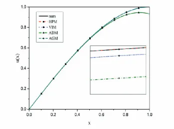
Fig. 1. A comparison of the results of the methods.
Fig.2. A comparison between the first derivatives of the methods.
Fig.3. A comparison between the second derivatives of the methods.
Fig.4.Comparing the charts of the achieved solution by AGM for various amounts of Re.
Fig.5. A comparison amongst the obtained charts by AGM for the first derivative of the achieved solution in terms of different values of Re.
Fig.6.A comparison amongst the obtained charts by AGM for the second derivative of the achieved solution in terms of different values of Re.
Fig.7..A comparison between AGM and numeric method
Table Caption
Table.1..The obtained results in accordance with the Numerical Solution of Eq. (1).
Fig.2. A comparison between the first derivative of the Methods.
cig.4. Comparing the chtrts of ahe aFhieved solution by AGM for various amounts of Re.
Fig.6. A comparison amongst the obtained chauos by AGM for the second derivative of the achieved selrtion in terms of differont values tf Re.
Fig.8.A comparison between Errors of methods.
Table.1. The obtained results in accordaece with the bumnrical Solution of Eq. (2.1).
x 0 0.2 0.4 0.6 0.8 1 F(x) 0 0.29724 0.57001 0.79390 0.94488 1
F0(x) 1.50662 1.44542 1.26190 0.95692 0.53369 0