Full-Reference and No-reference Image Blur Assessment Based on Edge Information

(1)

Vol. 2 (2012) No. 1 ISSN: 2088-5334

Full-Reference and No-reference Image Blur Assessment Based

on Edge Information

David B.L. Bong, Adeline S.L. Ng

Faculty of Engineering, Universiti Malaysia Sarawak, 94300 Kota Samarahan, Malaysia. E-mail:[email protected]

Abstract— Blur images are often subjected to the loss of high frequency content during acquisition, compression and multimedia transmission. Hence, objective blur assessment is implemented to identify and quantify image quality degradation by blurriness artifact in order to maintain and control the quality of the images. In this paper, objective full-reference and no-reference blur assessments using edge information are presented with the aim to provide computational models that can automatically measure the amount of blurriness artifact such as Gaussian blur on the images. The amount of Gaussian blur on an image, also known as the final blur measurement is determined by averaging the sum of edge width over all detected edges which satisfy the edge criteria. The final blur measurement for all test images based on full-reference and no-reference implementations are also validated with subjective results. The validation results show that the objective full-reference and no-reference blur assessments correlate closely to perceptual image quality.

Keywords— Edge; full-reference; Gaussian blur; no-reference .

I. INTRODUCTION

Along with the rapid advances in digital and multimedia imaging industry, digital images have been playing an increasingly important role in the communication of visual information. Unfortunately, these images can be degraded during acquisition, compression, transmission or even processing. Thus, a measure to the image quality is necessary to assess the degree of degradation. The method of measuring the degree of degradation is categorized into objective and subjective evaluations. Objective method is based on mathematical measure while subjective method relies on the perception of a selected group of human observers such as professionals or lay viewers. Objective image assessment is least preferable as the most reliable means to access the image quality is through subjective evaluation, where the quality of the image is evaluated by human. However, it is not an easy task to conduct a subjective evaluation image assessment because it is expensive and time-consuming [1]. Due to the limitations in subjective evaluation, researchers believed that it is useful to design objective method as long as it produces results that correlate closely with human visual system (HVS) [2]. There are 3 approaches to objective image quality assessment that can be considered such as

no-measurement and full-reference (FR) no-measurement [2]. A FR measurement requires complete availability of the original image while NR method accesses the distorted image without using any reference image. Meanwhile, RR method needs partial information of the reference image and it is a trade-off between both NR and FR methods.

Researchers have developed various perceptual image quality metrics where these metrics are used to measure the global distortion but a perceptual objective image quality analysis to measure a specific artifact such as blur is rarely found. Therefore, this paper aims to propose an objective blur assessment using edge information which correlates well with human visual perception based on FR and NR implementations.

II. BLUR ASSESSMENT

(2)

introduced to measure the blur image to determine the level of degradation so that it can be corrected to a certain extent to produce a better quality image and maintain the pleasure of human observers in viewing the image.

There also other researches in blur assessment such as a No-reference Quality Metric for Measuring Image Blur presented by E. Ong et al. [4] in 2003 using the gradients’ directions of each pixel in the image, The Blur Effect: Perception and Estimation with a New No-Reference Perceptual Blur Metric proposed by F. Crete et al. [5] in 2007 by comparing the variations between neighboring pixels while X. Wang et al. [6] published a Blind Image Quality Assessment for Measuring Image Blur in 2008 which is also based on edge gradient information. Although in [4] and [5], the researchers mentioned that their metrics correlate well with results obtained from subjective experiments but the correlation values are not reported. Moreover, in [6], the authors did not mention about validating their metric with subjective scores. However, the blur assessment using edge information presented in this paper which is based on the method implemented by P. Marziliano et al. [3] is highly correlated with subjective blur ratings when measuring on Gaussian blurred images. Based on Pearson linear correlation and Spearman’s rank order reported in [3], the metric has shown 96% correlation with its subjective evaluation.

Nevertheless, the blur measurement is applicable to numerous applications such as blur estimation in digital photography, image processing, printing or as a simple metric in comparing two images.

III.METHODOLOGY

A. Test Images

There are two sets of images used as test images. The first set consists of synthetically generated blur artifact on 29 RGB original images from LIVE database [7] using Gaussian blur lowpass filter of kernel size 15 × 15. Each of the images is blurred using Gaussian standard deviations, σ

∈ {0.4, 0.8, 1.2, 1.6, 2.0}. This set of images is used for blur assessment implementation in Section IV-A until Section IV-C.

In the second set, these test images are used for analysis in Section IV-D. There are 29 original images blurred using circular-symmetric 2-D Gaussian kernel of standard deviations ranging from 0.42 to 15 pixels by H. Sheikh et al. [8] to generate 145 blur images. Each source images has five blur images distorted with different standard deviation.

The total test image in each set is 174 images including original and distorted images. Fig. 1 shows some of the test images used for the blur assessment.

Fig. 1 Original test images: (a) bikes (b) carnival dolls (c) caps (d) church and capitol

B. NR Implementation

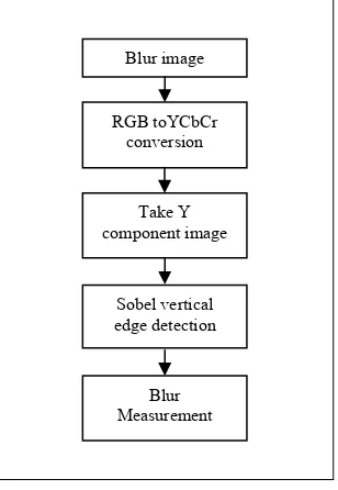
The blur image is converted to YCbCr color space as blurriness is measured on luminance (Y) component. The vertical Sobel edge detector is applied to the Y component image to determine the vertical edges. Blurriness can be measured on gray-level component by converting the RGB test image to grayscale image. The processing steps are illustrated in Fig. 2 below.

Fig. 2 Flow chart of NR implementation

C. FR Implementation

The original image is required for this implementation. Both original and blur images have to perform YCbCr color conversion. The vertical Sobel edge detector is then applied on the Y component image from the original image to obtain the location of the edges. As shown in Fig. 3, the blur measurement is based on the Y component of the blur image and edge locations detected from the original image.

(a) (b)

(c) (d)

Blur image

RGB toYCbCr conversion

Sobel vertical edge detection

Take Y component image

(3)

Fig. 3 Flow chart of FR implementation

D. Blur Measurement

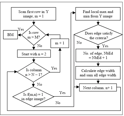
Fig. 4 Flow chart of blur measurement algorithm for an image having M

rows and N columns

The blur measurement algorithm is summarized in Fig. 4. First, scan the first row of the Y component image. For each edge detected from edge detection, the local minimum and maximum positions are determined. These positions are known as the start and end positions of the edge. They are also defined as the local extrema locations closest to the edge.

Fig 5 Edge falls on local maximum and local minimum positions

After determining the start and end positions, the edge must satisfy the edge criteria because experimentally, insignificant edges are detected from Sobel edge detection. For example, insignificant edges which are highlighted by the red circle on the line, fall on the same position as the start (local maximum) and end (local minimum) positions as illustrated in Fig. 5 above. These edges are not supposed to fall on such positions because it is not possible to obtain the edge width for these edges. Other types of insignificant edges are such that the edges fall on the start or end pixel position in some particular row in the image.

Thus, the edge criteria are introduced to overcome this problem. The edge is only accepted based on certain conditions as follows:

• An edge must reside in between a local minimum and a local maximum.

• An edge cannot fall on the start or end pixel position in every row of an image.

• An edge cannot fall on the same pixel position as the local minimum or local maximum.

Hence, once the detected edge satisfies the criteria, the edge width of the accepted edge is calculated. The edge width is given by the difference between the start and end positions. It is also known as the local blur measure for an edge location. The procedure of calculating the edge width and number of edges is repeated for every row in the image. The total blur measurement of a blur image is summarized as,

Blur metric (BM) = ∑Edge width

Total number of edges (1)

An example is shown in Fig. 6 below on calculating the edge width for an edge which falls on position P1. The edge width for this edge is given by the difference between P2 (start position) and P2′ (end position), which is 7 pixels for this example.

Yes

No

Yes

No

Yes

No

Calculate edge width and sum all edge width

Find local max and min from Y image

Does edge satisfy the criteria?

No. of edge, NbEd = NbEd + 1

Next column, n+ 1 BM

Scan first row in Y image, m = 1

Is row m > M?

Is column n > N – 1?

Is f(m,n) = 1 in edge image? Start with n = 2

m + 1

Yes No

Original image

Sobel vertical edge detection

Blur image

(4)

T imp A. I incr blur incr bec ima dec wid eve this Ma in F sub ther mea mea Bl M

Fig. 6 Calc

IV This section s plementation a

NR Blur Asse

It is clearly se reases with rriness artifa reases), the im come thicker r

age becomes creases. From dth and the d entually increa

s graph are arziliano et al.

Fig. 8. Both bjective evalua

re is a high asurement an asurement fol

Fig. 7 NR 2.964 0 2 4 6 8 10 12 14 0 Bl ur M easur e men t Blur Me

culating edge wid

V.RESULTS AN summarizes a and results fro

essment on Lu

een from the g the standard act increases mage become resulting in th

smoother, th equation (1) decrease of to ase the blur m

also validat [3] on the sa graphs appea ation conduct correlation ra nd human per

lows well wit

R blur assessment

46 3.2095

5.

0.4 Ga easurement ag

dth for an edge at

ND DISCUSSIO and discussed om each analy

uminance Com

graph in Fig. d deviation. s (standard es smoother. he increase of he number of , the increase otal number o measurement ted with the ame image wh ar to be simila ed by P. Mar ate of 96% b rception. This th subjective in

t results for bikes 4780

7.8011

0.8 1.2

aussian Blur (σ) gainst Gaussi

position P1

ON

the results fr ysis.

mponent

7 that the me This is true

deviation va Thus, the ed f edge widths. f detected ed e of sum of e of detected ed . The results e results by hich is illustra ar. Based on rziliano et al. between the b

s shows that nterpretation. test image 10.0203 11.8 1.6 2 )

an Blur (σ)

rom etric as alue dges As dges edge dges for P. ated the [3], blur the B. imp tha NR dis det blu So lar imp doe C. ass wit Th blu neg com blu of 554 2

Fig. 8 NR blur as

FR Implemen Based on th plementation at of NR imple

The variation R implementa storted image tected in the ur increases, it

bel filter. Als ger when the plementation, es not corresp

Fig. 9 Com

Analysis on N There are th sessment such 1) on graysc th the results he graphical re

ur measurem gligible. The mponent close ur measured o

the test image

0 5 10 15 0 Blur Measur ement Blur Me 12 11 10 9 8 7 6 5 4 O b je ctive M e as ur eme n t

0 0.2

ssessment results Marzilian

ntation he compariso

tends to prov ementation.

of the measu ation, the edg e while in FR

original imag t decreases th so, the edge w

level of blurr the increase pond to the num

mparison between

NR Blur Asses hree types of h as follows:

ale componen of NR blur esult in Fig. 1 ent between

graph of b ely follows th n grayscale co es.

0.4 0.8

Gaussia easurement a

2 0.4 0.6 0.8

G

for bikes test im no et al. [3]

on graph in vide lower m

urements is ex ge detector i FR implement ge. Thus, usin he number of e width for each ring is higher. e of the deg umber of edge

n NR and FR blu

ssment f analysis do

nt: This anal assessment o 10 shows that n two compo

blur measure he same patter omponent. Th

1.2 1.6

an Blur (σ) against Gauss

8 1 1.2 1.

Gaussian σ

age provided by P

Fig. 9, the metric values

xpected becaus s applied on tation, edges ng NR method

edges detected h detected edg

However, for gree of blurri

detected.

r assessment

one on NR

lysis is comp on Y compon t the differenc onent images ed on lumina rn of the grap his applies to m

2 2.4

ian Blur (σ)

.4 1.6 1.8

(5)

Fig. 10 Comparison between NR blur assessment on luminance component and grayscale component for bikes test image

2) using grayscale images: This analysis is to compare with the blur measurement in Section IV-C-1. Graphically, the results are identical as seen in Fig. 11.

Fig. 11 Comparison between NR blur assessment using grayscale image and RGB image represented by grayscale component of bikes test image

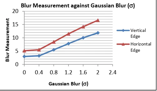
3) horizontal edge information: The NR blur measurement presented by P. Marziliano et al. [3] considers only vertical edges due to performance reasons. However, the blur assessment can be easily extended to horizontal edge detection. Fig. 12 shows that blur metric based on horizontal edge detection is higher than the metric value from vertical edge detection. This applies to most of the test images.

Fig. 12 Comparison between NR blur assessment based on vertical edge

D. Analysis using LIVE Database Gaussian Blur Images Below are the blur assessment implementations using blur images from LIVE database [7]. The result of each implementation is validated with subjective testing result (DMOS values) from LIVE database [7].

1) NR Implementation: The scatter plot in Fig. 13 shows a relatively high correlation between the objective and subjective results with R2_{equivalent to 0.81. R}2_{value close}

to 1 indicates excellent linear reliability and correlation.

Fig. 13 Correlation between NR normalized blur measurement and DMOS values

2) FR Implementation: Fig. 14 illustrates the blur measurement for all test images with respect to the subjective results. The blur metric performs well and the value of R2_{is 0.87 indicates high correlation.}

Fig. 14 Correlation between FR normalized blur measurement and DMOS values

3) Line fitting method (to obtain normalized blur measurement): This method is to align the linear graph of the objective results closer to the nonlinear graph of the subjective results. First, the difference between the blur measurement of the original image and blurred image is obtained. Then, the square root of the difference in measurement (SDBM) is calculated and represented as,

SDBM = BM − BM (2)

0 5 10 15

0 0.4 0.8 1.2 1.6 2 2.4

Blur

Measur

ement

Gaussian Blur (σ)

Blur Measurement against Gaussian Blur (σ)

Luminance Component

Grayscale Component

0 5 10 15

0 0.4 0.8 1.2 1.6 2 2.4

Blur

Measur

ement

Grayscale Image

RGB Image (Grayscale Representation)

0 5 10 15 20

0 0.4 0.8 1.2 1.6 2 2.4

Blur

Measur

ement

Vertical Edge Horizontal Edge

R² = 0.8084

0 20 40 60 80 100 120

0 50 100 150

DMO

S

Normalized Blur Measurement (NBM) DMOS against NBM for NR Implementation

R² = 0.8672

0 20 40 60 80 100

0 20 40 60 80

DMO

S

(6)

where, BMBLUR denotes the raw blur measurement of blur

images and BMORI is the raw blur measurement of original

image.

The graph of SDBM against DMOS values is then plotted for every blur level in the image and both lines are aligned using Microsoft Excel trendline function. A gain, α is obtained from the average of DMOS and SDBM line gradients. Thus, the gain is multiplied with SDBM values to acquire the normalized blur measurement (NBM) values.

E. Discussion

Based from the results, the blur metric increases with Gaussian blur standard deviation. The increase of degree of blurriness in an image produces a smoother image, hence this affects the number of detected edges to decrease and the edge width of each detected edge to increase. Thus, from equation (1), the blur metric eventually increases due to the increase of sum of edge width and the decrease of total number of edges.

Moreover, the metric values based on FR implementation are lower than that of the metric values from NR implementation. This is because in FR method, the increase in blur level does not affect the number of detected edges.

In both Section IV-C-1 and Section IV-C-2, the results indicate that the comparison graphs are similar. Meanwhile, Section IV-C-3, it is observed that the horizontal edge detection does not improve the measurements. For the analysis in Section III-D, the results from NR and FR blur assessments correlate closely to subjective results.

Concisely, the blur assessment has low computational complexity. The total computational time for measuring blur on all 174 test images in any method of implementation (NR or FR) is approximately 160 seconds. Hence, the elapsed time of measuring blur artifacts on an image is less than 1 second.

V. CONCLUSIONS

A low computational complexity objective blur assessment is successfully implemented to measure the degree of blurriness in an image. Different types of analysis are also carried out to evaluate the performance of the blur assessment. The results of the assessments are as well validated with subjective results where the validation indicates that there is a close correlation between the objective blur assessments with human perception.

As for further work, the blur assessment can be easily extended to digital video quality assessment to measure the level of blur in every consecutive frame in the video. The global blur measurement of a video will be the average of local blur measurement in every successive frame. Hence, the blur assessment can be improved so that is also applicable to real-time application. Besides that, blur identification algorithm is recommended to implement together with the blur assessment. Instead of measuring the amount of blur artifacts that present in an image, the type of blur that degrades the image can be identified so that user will have knowledge on which type of blur distorts the image quality. Finally, further research can be done on the blur assessment by measuring blurriness in color images on other color component such as hue instead of measuring on the luminance component.

ACKNOWLEDGMENT

The authors would like to acknowledge Faculty of Engineering, Universiti Malaysia Sarawak for the provision of research facilities.

REFERENCES

[1] Z. Wang, G. Wu, H. R. Sheikh, E. P. Simoncelli, E. –H. Yang, and A. C. Bovik, "Quality–aware images," IEEE Transactions on Image

Processing, vol. 15, no. 6, pp. 1680 – 1689, June 2006.

[2] Z. Wang, H. R. Sheikh, and A. C. Bovik, “Objective Video Quality Assessment,” in The Handbook of Video Databases: Design and

Applications, B Furht and O. Marqueseds, Eds. Boca Raton, FL:

CRC, 2003, pp. 1041 – 1078.

[3] P. Marziliano, F. Dufaux, S. Winkler, and T. Ebrahimi, “A no– reference perceptual blur metric,” in Proc. of the International

Conference on Image Processing, Rochester, NY, 2002, pp. 57 – 60.

[4] E. Ong, W. Lin, Z. Lu, X. Yang, S. Yao, F. Pan, L. Jiarrg, and F. Moscheni, “No–reference quality metric for measuring image blur,”

in Proc. of IEEE International Conference on Image Processing,

Sept. 2003, pp. 469 – 472.

[5] F. Crete, T. Dolmiere, P. Ladref, and M. Nicolas, “The blur effect: perception and estimation with a new no–reference perceptual blur metric,” in Proc. of SPIE on Human Vision and Electronic Imaging XII, San Jose, California, USA, Jan. 2007.

[6] X. Wang, B. Tian, C. Liang, and D. Shi, "Blind image quality assessment for measuring image blur," in Proc. of Congress on

Image and Signal Processing, 2008.

[7] H. R. Sheikh, Z. Wang, L. Cormack and A.C. Bovik, "LIVE Image Quality Assessment Database Release 2", http://live.ece.utexas.edu/res

earch/quality.

[8] H. R. Sheikh, M. F. Sabir and A. C. Bovik, "A statistical evaluation of recent full reference image quality assessment algorithms", IEEE

Transactions on Image Processing, vol. 15, no. 11, pp. 3440 – 3451,