Please cite this article as: M. R. Taheri, R. Esmaelzadeh, J. Karimi, Differential Flatness Method Based on Pre-set Guidance and Control Subsystem Design for a Surface to Surface Flying Vehicle, International Journal of Engineering (IJE), TRANSACTIONS C: Aspects Vol. 30, No. 6, (June 2017) 912-919
International Journal of Engineering
J o u r n a l H o m e p a g e : w w w . i j e . i r
Differential Flatness Method Based on Pre-set Guidance and Control Subsystem
Design for a Surface to Surface Flying Vehicle
M. R. Taheri, R. Esmaelzadeh*, J. Karimi
Malek Ashtar University of Technology, Aerospace Department, Tehran, Iran
P A P E R I N F O
Paper history:
Received 21 January 2017
Received in revised form 27 March 2017 Accepted 21 April 2017
Keywords: Nonlinear Systems Flat Differential Technique Preset Guidance Flatness Based Controller
A B S T R A C T
The purpose of this paper is to design a guidance and control system and evaluate the performance of a sample surface-to-surface flying object based on preset guidance with a new prospective. In this study, the main presented idea is usage of unique property of governor differential equations in order to design and develop a controlled system. Thereupon a set of system output variables have been examined by specific tests as candidate of flattened variables. It is proved that the dynamism of the studying system has a property of differential flatness. This property as a basement for observing all of the system dynamic variables could be a perfect option to remove lack of observability of nonlinear systems. According to the information gained in the procedure of flatness demonstrating, there was a similarity between the control command generating in feedback linearization and flat systems tests. This similarity led to the application of the flat systems technique for the mentioned control method. The guidance and control system suggested in this paper is able to follow a set of specific reference trajectories in order to target different ranges. This ability without recalculating controller gains could be done only by having the rate of rotate of flying object in middle phase of maneuver. To validate the proposed FBC for the studied problem, another usual control method has been investigated. For this purpose, the linear quadratic regulator as straight forward control method in optimal control field has been applied. This feature reveals full compatibility between controller block and reference trajectory generator block.
doi: 10.5829/ije.2017.30.06c.12
1. INTRODUCTION1
A variety of different methods have been presented in control and guidance systems recently [1]. These trajectories are usually stored in flight computer. The controller has such a design that could follow this trajectory [2]. Feedback linearization is one of the controller design methods for approaching to auto pilot. This method, which belongs to nonlinear control categories, is based on linearization of system error dynamics [3]. The control of signal command could be generated only by knowing all of the system state variables. This is the main disadvantage of the feedback linearization in such systems that not all of state variables are available.
*Corresponding Author’s Email: [email protected] (R.
Esmaelzadeh)
A sample of usage of this method has been shown in the literature [4]. In fact, observing and measuring all system state variables are not possible. Hence these variables should be estimated [5].
In these recent years, a technique has been presented which is based on a property in system dynamic structure named flat differential. This method has been used in many engineering fields such as robotics [6]. Also it has been used for guidance and control of re-entry vehicles [7] and satellites attitude control [8] in aerospace engineering. In this paper it was intended to design a sort of state observer by this technique. In this method there was no linearization in dynamic equations of system and fully nonlinear form of the equations were used in controller design process. By using feedback linearization method, the control command could be applied onto system. Finally, the error differential equations of the controlled system come in
the form of a linear differential set. Toloei et al. in their work optimized suspension system for one type of aircraft to achieve desirable response using linear controller and optimization algorithm [9-11].
Designing the autopilot of a surface-to-surface flying object which is based on flat differential property is the main goal in this study. The reference trajectory in this study has been produced by pre-set guidance generator in order to attack a fixed point.
2. FLAT DIFFERENTIAL DEFENITION
Many dynamic systems have a property in their structure named flat differential that equals to existence of a set of independent variables of system outputs and their combinations of derivatives. The number of flat variables exactly equals to the number of system control inputs. This option results in a square framework that all of the system variables and also all of the control inputs could be completely parameterized thanks to the flat variables. This method was expressed and developed by a French research group in 1992 [12]. The method introduction and some case studies have been mentioned in reference [13].
If a set of nonlinear differential equations are considered in general form:
(1)
where 𝑥 ∈ ℛ𝑛 expresses the state variables of system
and 𝑢 ∈ ℛ𝑚 expresses the control input of system,
which 𝑚 ≤ 𝑛. System 1 is called Flat System if an independent vector of outputs or their combinations in form of 𝐹 ∈ ℛ𝑚have been found in such a way that all
of the system variables and also all of the control inputs could be expressed as separated functions of these flat variables and the finite number of their derivatives. In the other word, the diffinition of flatness could be expressed as two conditions in mathematical form as follow:
(2)
where, S is an integer elemental vector which expresses the order of derivatives of variables S = (S1, S2, … , Sm).
And also F is a function of x, u and infinite number of u such as below:
(3)
where, r is a positive integer.
3. THE SYSTEM DYNAMICS
The issue, which is concentrated in this paper, is the ground-to-ground flying object control to attacked fixed
targets in different ranges. For this purpose the ground-to-ground flying object uses a predetermined guidance program which is able to attack in different ranges by changes in one of the parameters of reference guidance generator block.
Since the main focus of this article has been on the utilization of FBC and compatibility between control and guidance block, effort has been made to make the selected dynamic model as simple as possible. A few important assumptions are as follow:
Dynamics of rigid body in-plane, 3DOF has been considered.
All of noise signals coming from the environment condition have been ignored.
Curvature of the earth has been ignored.
Standard atmospheric model has been considered. Flight dynamic equations are available by applying Newton’s second law on the assumed model [14, 15]. In this issue the velocity coordinate is the best option to express flight equations and differential flatness property. This coordinate has a unique property for expressing the flight equations’ of center of mass and rotational equations of the flying object around the center of mass. Hence it is able to perform a successful test of a flat system. Dynamic equations of the system, including kinetic and kinematic equations are listed below. Kinetic equations:
(4)
where V, , q are kinetic variables which respectively show center of mass velocity of the flying object, the path angle and angular velocity. q
shows the dynamic pressure,
m I
,
yy are respectively mass and moment of inertial of the flying object. Also T shows the flying object thrust force as the first control variable.(5)
,
D L and Mare respectively aerodynamic forces (Drag and Lift) and aerodynamic moment which can be obtained by aerodynamic dimensionless coefficients
(C C CD, L, M) and S shows the aerodynamics cross
section area.
It should be noticed that aerodynamic coefficients used for the considered dynamic model could be obtained in the form of functions of dimensionless variables such as Mach number, angle of attached, α, the rotation rate of the flying object body and also elevator angle, δe, as the second control variables. All of these factors are taken from reference [16].
( , ) x f x u
( )
( 1)
( , , ,..., )
( , , ,..., )
s s
X F F F F
u F F F F
( ) ( , , , ,..., r ) F h x u u u u
sin( ) cos( )
cos( ) sin( )
yy
mV mg T D
mV mg T L
M q
I
, ( , )
, ( , )
, ( , , , )
D D L
L D
M M e
D qSC C f Mach C L qSC C f Mach M qScC C f Mach q
Kinematic equations:
(6)
which x and z in the above equation represent the center of mass position of flying object on the vertical flight plane.
4. FLATNESS PROOFING
In this section it will be proved that the dynamic structure of the system is flat if the candidate flat variables can satisfy two tests of flatness property. These two basic tests indicate that each of the system state variables (as the first test) and each of the control commands (as the second test) should be able to be expressed as separated functions of flat variables and a finite number of their derivatives. Since, the case study is considered in this article, the position variables of center of mass were selected as the candidate flat variables. Therefore, one can find these functions by following the procedure below.
First test: The functions of system state variables. Based on the unique feature of velocity frame that has been explained, determination of each function of 𝜙𝑖, which i
equals to state variables of systems, is possible.
(7)
where the derivatives of the above functions will be needed to express attached angle.
(8)
Also the derivative of attached angle will be needed to express the rate of rotation of flying object.
(9)
By following the above procedure all of the state variables of the system could be expressed as functions of flat variables and their finite derivatives up to third order. Hence, the selected flat variables satisfy the first test of flatness successfully.
Second test: The functions of control inputs.
The purpose of this test is to provide all the control inputs of system. Determination of each function of 𝜓𝑖, which i
equals to control inputs, is possible only by a perfect knowledge of system equations.
(10)
Derivative of rate of rotation of vehicle is needed to express another control input.
(11)
By following the above procedure, all of the control inputs of system could be expressed as functions of flat variables and their finite derivatives up to the fourth order. Hence the selected flat variables satisfy the second test of flatness property successfully and then can be defined as a set of flat variables of this system. These independent set of variables could be used in controller design procedure that mentioned in next section.
5. FLATNESS BASED CONTROLLER
Many different methods have been proposed in order to achieve a design of controller for nonlinear dynamic systems. The selected method in this article was based on using flat systems technique in observing all the system variables. The generated control command applied to the plant in such a way that system error dynamics have been linearized. Hence, the stability of system has been guaranteed. The main reason of using flat systems technique is that feedback linearization method relies on two facts.
First, expression of control inputs as functions of flat variables and a finite number of their high order derivatives is very similar to essential command control in the feedback linearization method. Second, expression of the entire system variables in such a form that eliminates main restriction of mentioned method which is unavailability of all the system variables. Structure of designed controller based on flatness technique contains combination of two separated blocks, a nominal feed forward control and a feedback stabilizer block. As a matter of fact, the concept of flatness based control (FBC) allows designing the control as explained before. It can be seen in Figure 1 that feed forward control provides a nominal input trajectoryu t( )which forces the system to the desired output trajectoryy t( ) in the nominal case. By this technique, the command control and the disturbance response can be designed separately [17].
cos( ) sin( ) x V z V q 2 2 (1) (1)
1 1 2
1
1 (1) (1)
2
2 1 2
( , )
tan ( , )
V x z F F
x F z z F F F x
(1) (2) (1) (2)
1 1 1 2 2
(1) (2) (1) (2)
2 1 1 2 2
1 (1) (2) (1) (2)
3 1 1 2 2
( , , , )
( , , , )
cos( )
tan ( ) ( , , , )
sin( )
V F F F F
F F F F
mV mg L
F F F F
mV mg D
(1) (2) (3) (1) (2) (3)
3 1 1 1 2 2 2
(1) (2) (3) (1) (2) (3)
4 1 1 1 2 2 2
( , , , , , )
( , , , , , )
F F F F F F
q F F F F F F
(1) (2) (1) (2)
1 1 1 2 2
sin( )
( , , , )
cos( )
mV mg D
T F F F F
(1) (4) (1) (4)
4 1 1 2 2
(1) (4) (1) (4)
2 1 1 2 2
( ,..., , ,..., ) 1 ( ,..., , ,..., ) 2 e yy
e M Mq
M
q F F F F
q I qc
C C F F F F
C qSc V
Figure 1.Block diagram of flatness based controller
Accordingly with substituting the highest derivative terms of flat variables by following form, we can achieve mentioned control command.
(12)
For this case study the 𝜈 control command was regarded as below:
(13)
This scheme of controller has all three properties of PID controller for compensating errors. With substituting above control command in governing equations, the dynamics of error of system will be drivable as below:
(14)
where in above equations e expresses the error signal between actual and reference flat variables. Finally the equation of system error dynamics could be used for calculating appropriate gains corresponding to desired reference trajectories.
6. REFERENCE GUIDANCE TRAJECTORY
In this paper the reference trajectory based on low guidance was generated to attack fixed targets. In this problem it was assumed that the target has been fixed in 200 kilometer far from the start point and reference trajectory of flying object was partitioned to five maneuvers with specific characteristic. Each of these quintet maneuvers generated in guidance block could be expressed in general function form as follows:
(15)
where, a and m express linear constant acceleration of center of mass and rate of rotation of path angle. And
𝑉0 and 𝛾0express the initial conditions of velocity profile
and path angle profile. Table 1 contains this constant corresponding to each maneuver. In this article, the provided reference trajectory form has the ability to
attack any different fixed ranges only by knowing the third interval time of maneuver. The guidance block has been programmed in such a form that can calculate this parameter by interring the desired range as input. In guidance block design, the main idea of this parameter was based on very small error of tracking in the third maneuver. Hence, attacking different ranges will be possible with the same final error. This property helps us to avoid recalculating the controller gains for different reference trajectories. In the other word, this property reveals full computability between guidance block and controller block to achieve a system with no need to recalculating gains for attacking indifferent ranges.
7. SIMULATION AND RESULTS
To show the performance of guided and controlled system which are proposed in this article, a comprehensive simulation has been carried out in
MATLAB/Simulink. In this simulation the
environmental disturbances and other uncertainties were neglected. However, many physical limitations of the selected vehicle such as allowable deflection range of the control surface and rate of propellant consumption were considered. All of the environmental parameters such as air density, sound velocity and gravity acceleration were considered based on standard models. The following figures show the simulation results with FBC.
As illustrated in Figures 2 and 3, the flat outputs have been tracked with an acceptable error. The maximum tracking error for
x
is about 68 meters and maximum error forz
is about 45 meters. These values reach zero in third stage which is ideal for guidance block to attack different range.As shown in Figures 6 and 7, the linear velocity of mass center and path angle have been tracked with an acceptable error. The maximum tracking error for V is about 2 meters per second and maximum error for path angle is about 0.6 degrees. Observations of dynamics variables have been shown in Figures 8 and 9 in which the area obtained from flatness is based on nonlinear observer within maneuver.
TABLE 1. Maneuver parameters
Maneuver parameters
Nomencl ature
Stage 1
Stage 2
Stage 3
Stage 4
Stage 5
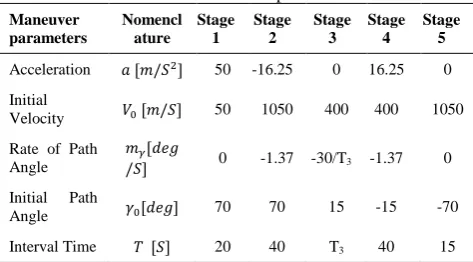
Acceleration 𝑎 [𝑚/𝑆2] 50 -16.25 0 16.25 0
Initial
Velocity 𝑉0 [𝑚/𝑆] 50 1050 400 400 1050
Rate of Path Angle
𝑚𝛾[𝑑𝑒𝑔
/𝑆] 0 -1.37 -30/T3 -1.37 0
Initial Path
Angle 𝛾0[𝑑𝑒𝑔] 70 70 15 -15 -70
Interval Time 𝑇 [𝑆] 20 40 T3 40 15
( 1)
( 1) ( ) ( )
Re Re Re
0
( )
s
s
s j j
f j f al
j
F
F K F F
Re Re Re Re Re Re Re
0
( ) ( ) ( )
f
t t
f d f al p f al i f al t
F K F F K F F K F F dt
0
Re Re
0
f
t t
d p i
t al f
e K e K e K edt
e F F
0 0
ref ref
V at V
m t
Figure 2. The error of x posision of center of mass
Figure 3. The error of z posision of center of mass
Figure 4. The derivative of error of x posission of center of mass
Figure 5. The derivative of error of z possision of center of mass
Figure 6. The velocity of center of mass
Figure 7.The path angle
Figure 10 shows in plane trajectory of flying object over five stages.
Figure 11 shows the elevator deflection control command of flying object which is constrained by physical achievable deflection of control surfaces. Figure 12 shows the thrust control command. As shown in these figures, the aerodynamic deflection and thrust control commands have smooth behavior in the third stage of maneuver. In total, all of the reference variables trajectories have been tracked with acceptable errors. This indicates the ability of flatness technique to observe all of the state variables.
Figure 8. The body rate of rotate
0 100 200 300 400 500
-60 -40 -20 0 20 40 60
Time [sec]
eX
[m]
0 100 200 300 400 500
-50 -40 -30 -20 -10 0 10 20 30
Time [sec]
eZ
[m]
0 100 200 300 400 500
-40 -20 0 20 40
Time [sec]
edot
X
[m/s]
0 100 200 300 400 500
-40 -20 0 20 40
Time [sec]
edot
Z
[m/s]
0 100 200 300 400 500
0 200 400 600 800 1000
t [sec]
V [m/
s]
V Reference V
Real
0 100 200 300 400 500
-80 -60 -40 -20 0 20 40 60 80
t [sec]
[deg]
Reference
Real
0 100 200 300 400 500
-30 -20 -10 0 10 20 30 40
t [sec]
q [deg/s]
q
Reference
q
Figure 9.The angle of attached
Figure 10. Inplane trajectory of center of mass
Figure 11. Elevator deflection control command
Figure 12. Thrust control command
For example the maximum error of attached angle in the third stage of maneuver shown in Figure 9 does not exceed from two degrees. Note that, almost all of the state variables have a very small error at the end of third
stage. Also it should be mentioned that the final error of attacking the target is about three meters. This final attacking error is fixed for a wide interval of fixed ranges.
8. VALIDATION OF THE PROVIDED FBC
To validate the proposed FBC for the studied problem, another usual control method has been investigated. For this purpose, the linear quadratic regulator as straight forward control method in optimal control field has been applied. Accordingly in order to achieve the LQR based tracker, as a basement of comparison and validation, we have to carry out the following procedure [18]. First, trim parameters of flight in desired reference should be determined. Also the linearization of governing equations around the different working points in reference trajectories is another important work that should be done carefully. As the final step in this procedure, we have to obtain the appropriate state feedback gains and then apply these gains into close loop scheme.
The above procedure of designing LQR tracker has been done on the studied problem. Each method has shown the tacking error of flat variables in Figures 13 and 14.
As shown in Figure 13, the tracking error of velocity by flatness based controller has an acceptable behavior compared with LQR controller. The error of velocity by FBC method is bounded with 2 m/s while this value in LQR method exceeds from 9 m/s.
Figure 13. Comperssion between velocity errro in FBC and LQR methods
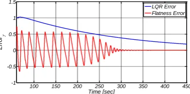
Figure 14. Error of 𝛾, by FBC and LQR methods
0 100 200 300 400 500
-30 -20 -10 0 10 20
t [sec]
[deg]
Reference Real
0 0.5 1 1.5 2
x 105
0 1 2 3 4
x 104
X [m]
Z [m]
Trajectory
Reference
Trajectory
Real
0 100 200 300 400 500
-30 -20 -10 0 10 20 30
t [sec]
Ele
v
a
to
r
[d
e
g
]
0 100 200 300 400 500
0 1 2 3
4x 10
5
t [sec]
T
h
ru
s
t
[
N
]
100 150 200 250 300 350 400 450
-4 -2 0 2 4 6 8 10
Time [sec]
Error
v
LQR Error Flatness Error
100 150 200 250 300 350 400 450
-1 -0.5 0 0.5 1 1.5
Time [sec]
Error
Furthermore the path angle as the main characteristic of the maneuver by FBC method has been tracked namely after passing the second stage by FBC method. As shown in Figure 14 the tracking error of this parameter is bounded with 0.6 deg/s.
In addition the LQR tracker needs to follow the boring mentioned procedure to obtain the state feedback gains in comparison to FBC. The above results show the advantage of tracking error in FBC method. Furthermore, the main defect of LQR which is the assumption of accessibility of all of the state variables still remains.
9. CONCLUSION
In this research, the use of flatness technique of nonlinear system has been applied into design of coupled guidance and controlling a surface-to-surface flying object. Our proposed approach does not need to recalculate controller gains hence a set of specific reference trajectories could be tracked in order attack the target different ranges. This feature provides full compatibility between controller block and pre-set guidance reference generator block. Furthermore, the presented method could be considered as a perfect observer for those nonlinear systems in which not all of the state variables are available. The investigated method was validated with LQR optimal method, the error results of the two methods show the advantage of using FBC.
10. FURTHER WORKS
As a future work in continuing and completing this article, it would be interesting to apply FBC method to track reference trajectories which are based on proportional guidance (PG). This combination of FBC and PG method could be investigated for neutralizing any unpredicted attacks. This new approach also could be considered to be evaluated by various analytical methods such as Mount Carlo in different target maneuverings.
11. REFERENCES
1. Shima, T., Idan, M. and Golan, O.M., "Sliding-mode control for
integrated missile autopilot guidance", Journal of Guidance,
Control, and Dynamics, Vol. 29, No. 2, (2006), 250-260.
2. Li, C., Jing, W., Wang, H. and Qi, Z., "Development of flight
control system for 2d differential geometric guidance and
control problem", Aircraft Engineering and Aerospace
Technology, Vol. 79, No. 1, (2007), 60-68.
3. Li, C., Jing, W., Wang, H. and Qi, Z., "Application of 2d
differential geometric guidance to tactical missile interception", in Aerospace Conference, IEEE, (2006), 6-15.
4. Graichen, K. and Zeitz, M., "Feedforward control design for
finite-time transition problems of nonlinear systems with input
and output constraints", IEEE Transactions on Automatic
Control, Vol. 53, No. 5, (2008), 1273-1278.
5. Brown, A.S. and Hardiman, D.F., "Applications of nonlinear
estimation techniques", COMPEL-The International Journal
for Computation and Mathematics in Electrical and Electronic
Engineering, Vol. 28, No. 2, (2009), 286-303.
6. Tang, C.P., "Differential flatness-based kinematic and dynamic
control of a differentially driven wheeled mobile robot", in Robotics and Biomimetics (ROBIO), IEEE International Conference on, IEEE., (2009), 2267-2272.
7. MORIO, V., "Design and development of an autonomous
guidance law by flatness approach", Vol., No.
8. Louembet, C., Cazaurang, F., Zolghadri, A., Charbonnel, C. and
Pittet, C., "Design of algorithms for satellite slew manoeuver by flatness and collocation", in American Control Conference,. ACC'07, IEEE., (2007), 3168-3173.
9. Toloei, A., Aghamirbaha, E. and Zarchi, M., "Mathematical
model and vibration analysis of aircraft with active landing gear
system using linear quadratic regulator technique",
International Journal of Engineering-Transactions B:
Applications, Vol. 29, No. 2, (2016), 137-144.
10. Toloei, A., Zarchi, M. and Attaran, B., "Oscillation control of aircraft shock absorber subsystem using intelligent active performance and optimized classical techniques under sine wave
runway excitation", International Journal of Engineering,
Transactions C: Aspects, Vol. 30, No. 3, (2016), 1167-1174.
11. Toloei, A.R., Zarchi, M. and Attaran, B., "Optimized fuzzy logic for nonlinear vibration control of aircraft semi-active shock
absorber with input constraint", International Journal of
Engineering, Transactions C: Aspects, Vol. 31, No. 3, (2016),
1300-1306.
12. Fliess, M., Levine, J., Martin, P. and Rouchon, P., "On differentially flat nonlinear systems", in IFAC SYMPOSIA SERIES., (1992), 159-163.
13. Fliess, M., Lévine, J., Martin, P. and Rouchon, P., "Flatness and defect of non-linear systems: Introductory theory and examples",
International Journal of Control, Vol. 61, No. 6, (1995),
1327-1361.
14. Eshelby, M.E., "Aircraft performance: Theory and practice, American Institute of Aeronautics and Astronautics, (2000).
15. Taheri, M.R., Soleymani, A., Toloei, A. and Vali, A.R., "Performance evaluation of a high-altitude launch technique to
orbit using atmospheric properties", nternational Journal of
Engineering, Transactions A: Basics, Vol. 20, No. 1, (2013),
333-340.
16. Sutton, F.B. and Martin, A., "Naca research memorandum", (1951).
17. Hagenmeyer, V., "Robust nonlinear tracking control based on
differential flatness", at-Automatisierungstechnik Methoden
und Anwendungen der Steuerungs-, Regelungs-und
Informationstechnik, Vol. 50, No. 12/2002, (2002), 615-622.
18. Donald, K., "Optimal control theory: An introduction", Mineola,
Differential Flatness Method Based on Pre-set Guidance and Control
Subsystem Design for a Surface to Surface Flying Vehicle
TECHNICAL NOTE
M. R. Taheri, R. Esmaelzadeh, J. Karimi
Malek Ashtar University of Technology, Aerospace Department, Tehran, Iran
P A P E R I N F O
Paper history:
Received 21 January 2017
Received in revised form 27 March 2017 Accepted 21 April 2017
Keywords: Nonlinear Systems Flat Differential Technique Preset Guidance Flatness Based Controller
ديكچ ه
زا يتياده ريسم يور رب حطس هب حطس هدنرپ مسج کي لرتنک و تياده متسيس يحارط هب ديدج يدرکيور اب هلاقم نيا هدش نييعت شيپ م
ي دزادرپ يليسنارفيد حيطست يگژيو زا هدافتسا رب ينتبم هتشون نيا رد هدش هداد طسب و هئارا يلصا هديا .
عجرم يتياده ريسم بيقعت يارب مزلا يلرتنک روتسد ديلوت دنور رد متسيس کيمانيد م
ي دشاب زا . اي ن ور هتسد ا ياهريغتم زا ي
طسوت ،حطسم ياهريغتم دزمان ناونع هب متسيس يجورخ نومزآ
اه تابثا و هتفرگ رارق قيقحت و يسررب دروم حرطم ي
م ي دوش يليسنارفيد حيطست تيصاخ ياراد هعلاطم دروم متسيس کيمانيد هک م
ي دشاب دوخ هک يگژيو نيا . انب گنس
يارب يي
هدهاشم بوسحم متسيس يکيمانيد ياهريغتم هيلک ي م
ي دوش ، م ي دناوت مدع ندومن فرطرب رد يبسانم هنيزگ ور
ي ت ذپ ي ر ي
س ي متس اه تسد هب حطسم ياهريغتم تابثا ريسم رد هک يتاعلاطا رب هيکت اب ساسا نيا رب .دشاب حرطم يطخريغ ي
م ي آ ي د م ي ناوت نومزآ و دروخسپ يزاس يطخ شور رد يلرتنک روتسد ديلوت رد يهباشت ياه
س ي متس اه هک تفاي حطسم ي
کينکت زا هدافتسا هب رجنم س
ي متس اه داي يلرتنک شور رد حطسم ي هدش
م ي دوش رد هدش داهنشيپ لرتنک و تياده متسيس .
نداد رارق فده يارب يتياده عجرم ياهريسم زا يصاخ هتسد بيقعت تيلباق هلاقم نيا اهدرب
رد کمک هب اهنت ار توافتم ي
لرتنک هرهب بيارض ددجم هبساحم هب زاين نودب و رونام ينايم زاف رد هدنرپ مسج کي شخرچ خرن نتشاد رايتخا دننک
اراد ه
م ي دشاب لرتنک کولب لماک قابطنا تيلباق هدننک نايب يگژيو نيا . رد يتياده ريسم هدننک ديلوت کولب اب هدننک
مرف اه ناسکي ي
عجرم ريسم م
ي دشاب .