*Corresponding author: Shenbaga Devi S ISSN: 0976-3031
ON CHANGING BEHAVIOR OF EDGES OF SOME SPECIAL CLASSES OF GRAPHS II
Shenbaga Devi
1
Aditanar College of Arts
2
V.O.C. College, Thoothukudi 628 008 Tamil Nadu, India
DOI: http://dx.doi.org/10.24327/ijrsr.
ARTICLE INFO ABSTRACT
Let =
Then
graph that admits a Near Skolem difference mean labeling is called a Near Skolem difference mean graph. paper, a new parameter
INTRODUCTION
We consider only finite, undirected and simple graphs in this paper. The vertex set and the edge set of a graph
by ( ) and ( ) respectively. For standard terminology and notations, we follow Harary (1) and for graph labeling, we refer to Gallian (2).
In this paper, a Near skolem difference mean graph investigated and a new parameter is introduced to find the minimum number of edges that should be
convert the non- near skolem difference mean graph near skolem difference mean graph ∗.
Definition: The fan graph ( ≥ 2) is obtained by joining all vertices of (Path of n vertices) to a further vertex
center and contains ( + 1) vertices and (2
is, = + .
Definition: The shadow graph ( ) of a connected graph constructed by taking two copies of say
vertex ′ in ′ to the neighbours of the corresponding vertex in ".
Available Online at
International
Vol. 9, Issue,
Copyright © Shenbaga Devi S and Nagarajan A Creative Commons Attribution License, which permits the original work is properly cited.
Article History:
Received 24th December, 2017 Received in revised form 13th
January, 2018 Accepted 8th February, 2018 Published online 28th March, 2018
Key Words:
Fan graph, Shadow graph, Jewel graph, splitting graphs, Near Skolem Difference Mean graphs, Near Skolem Difference Mean labeling.
Research Article
ON CHANGING BEHAVIOR OF EDGES OF SOME SPECIAL CLASSES OF GRAPHS II
Shenbaga Devi S
1* and Nagarajan A
2Aditanar College of Arts and Science, Tiruchendur 628 215 Tamil Nadu, India
V.O.C. College, Thoothukudi 628 008 Tamil Nadu, India
DOI: http://dx.doi.org/10.24327/ijrsr.2018.0903.1840
ABSTRACT
Let be a ( , ) graph and : ( ) → {1,2, … , + − 1, +
= , the induced edge labeling ∗is defined as follows:
Then is called Near Skolem difference mean labeling if ∗( ) are all distinct and are from
graph that admits a Near Skolem difference mean labeling is called a Near Skolem difference mean graph. paper, a new parameter is introduced and verified for some graphs.
We consider only finite, undirected and simple graphs in this paper. The vertex set and the edge set of a graph are denoted For standard terminology and notations, we follow Harary (1) and for graph labeling, we refer
In this paper, a Near skolem difference mean graph is is introduced to find the deleted from to near skolem difference mean graph into a
is obtained by joining all (Path of n vertices) to a further vertex called the
− 1) edges. That
of a connected graph is
′ and ". Join each to the neighbours of the corresponding vertex "
Definition: For a graph , the splitting graph which is denoted by ( ) is obtained by adding to each vertex
′ such that ′ is adjacent to every vertex that is adjacent in .
Definition: The Jewel is the graph with vertex set
{ , , , , : 1 ≤ ≤ }
( ) = { , , , , ,
MAIN RESULT
Definition: A graph = ( ,
said to have Nearly skolem difference mean labeling if it is possible to label the vertices
from {1,2, … . . , + − 1, +
edge e = uv , is labeled as is even and
is odd. The resulting labels of the edges are distinct and are from {1, 2, …
Near skolem difference mean labeling is called a Near skolem difference mean graph.
| ( )
f u
f v
( ) |
|
f u
( )
f v
( ) |
Available Online at http://www.recentscientific.com
International Journal of Recent Scientific Research
, Issue, 3(J), pp. 25334-25339, March, 2018
Shenbaga Devi S and Nagarajan A, 2018, this is an open-access article distributed under the terms of the Creative Commons Attribution License, which permits unrestricted use, distribution and reproduction in any medium, provided
CODEN: IJRSFP (USA)
ON CHANGING BEHAVIOR OF EDGES OF SOME SPECIAL CLASSES OF GRAPHS II
Tamil Nadu, India
V.O.C. College, Thoothukudi 628 008 Tamil Nadu, India
+ + 2} be an injection. For each edge
are all distinct and are from {1,2,3, … . }. A graph that admits a Near Skolem difference mean labeling is called a Near Skolem difference mean graph. In this
, the splitting graph which is denoted is obtained by adding to each vertex , a new vertex is adjacent to every vertex that is adjacent to
is the graph with vertex set ( ) =
and edge set
, , 1 ≤ ≤ }.
) with vertices and edges is said to have Nearly skolem difference mean labeling if it is possible to label the vertices xÎV with distinct elements ( )
+ + 2} in such a way that each , is labeled as ∗(e) =| ( ) ( )| if
is even and ∗(e) =| ( ) ( )| if is odd. The resulting labels of the edges are
… … . , }. A graph that admits a Near skolem difference mean labeling is called a Near skolem
International Journal of
Recent Scientific
Research
Definition: Let be a non-near skolem difference mean graph. Then the parameter of a graph
minimum number of edges to be deleted from a G, so that the resulting graph is Near skolem difference mean.
Proposition: Let G be a non-Near skolem difference mean graph.
Then = ( ) ≥ − − 2, (where
edges to be removed from G to make it Near skolem difference mean graph).
Proof: Let ∗ be the graph obtained from G, by removing k edges of G.
Then, | ( ∗) | = | ( )| = and | ( ∗)
− .
Let be a Near skolem difference mean labeling of that
: ( ∗) ⟶ {1,2, . . , + − − 1, + −
Let ∈ ( ∗) such that ∗( ) = − .
Then, | ( ) ( )| = – .
This implies | ( ) − ( )| = 2 − 2 − 1. This implies ( ) = 2 − 2 − 1 + ( ).
≥ 2 − 2
But, ( ) ≤ + − + 2.
This implies 2 − 2 ≤ ( ) ≤ + − +
This implies − ≤ + 2
And hence ≥ − − 2.
This is true even if, | ( ) ( )| = q – k.
Hence in both cases, ( ) ≥ − − 2.
Theorem: ( ) = − − 2 = 2 −
Proof: By Preposition, ( ) ≥ −
Let ∗be the graph defined by
∗= ( ) − { , / 3 ≤ ≤ −
where ( ∗) = { , / 1 ≤ ≤ } and
( ∗) = { , /1 ≤ ≤
− 1}⋃{ , , , }.
Then | ( ∗)| = 2 and | ( ∗)| = 2 + 2.
Let : ( ∗) → {1,2, … ,4 + 1, 4 + 4} be defined as follows:
( ) = 1
( ) = 4 + 4
( ) = − 1. ≡ 1( 2), 3 ≤
4 + 5 − , ≡ 0( 2), 3 ≤
( ) = 2 + 5 − , ≡ 1( 2), 1 ≤
2 + 4 + , ≡ 0( 2), 1 ≤
Let ∗ be the induced edge labeling of . Then,
∗( ) = 2 + 3 − , 1 ≤ ≤ − 1.
∗( ) = , 1 ≤ ≤ − 1.
∗( ) = + 3 ∗( ) = + 1 ∗( ) = ∗( ) = + 2
The induced edge labeling are all distinct and are
2}.
Then ∗ is a Near Skolem Difference Mean graph.
near skolem difference mean is defined as the minimum number of edges to be deleted from a G, so that the resulting graph is Near skolem difference mean.
Near skolem difference mean
is the number of edges to be removed from G to make it Near skolem difference
be the graph obtained from G, by removing k
| = | ( )| − =
be a Near skolem difference mean labeling of ∗, such
− + 2}.
+ 2.
6 for ≥ 4.
− 2 = 2 − 6.
− 1}.
be defined as follows:
≤
≤ .
≤ ≤
. Then,
The induced edge labeling are all distinct and are {1,2, … ,2 +
is a Near Skolem Difference Mean graph.
Hence, ( ) = 2 − 6
Example: Near skolem difference mean labeling of edge deleted graphs obtained from
fig 1 and fig 2 respectively.
Theorem: ( ) ≥ − − 2
the Jewel graph.
Proof: By Preposition, ( )
( ) = 2 + 12 ( ) = 2 + 9
( )=1
( ) = 3
( ) = 2 + 9 − 2 , 1 ≤
( ) = 9
( ) = 5
Let ∗ be the induced edge labeling of
∗( ) = + 6 ∗( ) = + 4 ∗( ) = + 5 ∗( ) = + 3
∗( ) = 4
∗( ) = 2
∗( ) = + 3 − , 1 ≤
∗( ) = 3
∗( ) = 1
The induced edge labeling of
{1,2, … , + 6}.
Hence, ( ) = − 2, for
Therefore ∗ a is Near Skolem Difference Mean graph.
Example: Near skolem difference mean labeling of the edge deleted graphs ∗ obtained from the Jewel graph for
= 6 are given in fig 3 and fig 4 respectively.
1 36 2 33
20 22 18 24
37
1 40 2
22 24 20 26
6 for ≥ 4.
Near skolem difference mean labeling of edge deleted graphs obtained from ( )and ( ) are given in
2 = − 2 for ≥ 3, where is
( ) ≥ − − 2 = − 2.
≤ − 2.
be the induced edge labeling of . Then,
≤ − 2
The induced edge labeling of ∗ are all distinct and are
≥ 3.
a is Near Skolem Difference Mean graph.
Near skolem difference mean labeling of the edge obtained from the Jewel graph for = 5 and are given in fig 3 and fig 4 respectively.
Fig 1
Fig 2
4 31 6 29
16 26 14 28
14 8
4 35 6 33
International Journal of Recent Scientific Research Vol. 9, Issue, 3(J), pp. 25334-25339, March, 2018
Theorem: ( ) = − − 2 = − 4 for ≥ 5 where is the graph ( , ).
Proof: By Preposition, ( ) ≥ − 4. Let ∗be the graph defined by
Let ∗= − { / 1 ≤ ≤ − 4} where
Let ( ∗) = { , , , / 1 ≤ ≤ }
and
( ∗) = { , , / 1 ≤ ≤ , − 3 ≤ ≤ }.
Then | ( ∗)| = 2 + 2 and | ( ∗)| = 2 + 4.
Let : ( ∗) → {1,2, … ,4 + 5,4 + 8} be defined as follows:
( ) = 4 + 8.
( ) = 2 − 1, 1 ≤ ≤ .
( ) = 2 .
( ) = 2 − 1 + 2 , 1 ≤ ≤ .
Let ∗ be the induced edge labeling of . Then,
∗( ) = 2 + 5 − , 1 ≤ ≤ .
∗( ) = + 5 − , 1 ≤ ≤ .
∗( ) = + 1 − , − 3 ≤ ≤
.
The induced edge labels are all distinct and are {1,2, … ,2 + 4}.
Then the edge deleted graph ∗ is Near skolem difference mean for ≥ 5.
Hence, ( ) = − 4.
Example: Near Skolem Difference Mean labeling of the graph
∗is given below in fig 5
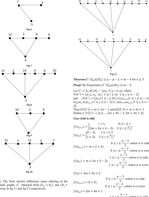
Theorem: The graph
( + ) =
− − 2 = − 4, ≥ 7
1 = 2, 3 2 = 4, 5 3 = 6
for ≥ 5.
Proof: By Preposition, ( + ) ≥ − 4.
Let ∗ be the graph obtained from + ℎ ( ∗) =
{ , /1 ≤ ≤ }.
and ( ∗) = { , , , , / 1 ≤ ≤ − 1}
. Then | ( ∗)| = + 1 and | ( ∗)| = + 3.
For = 2,4,6, the Near Skolem Difference Mean labeling of
∗ for = 2,4,6 are as shown in fig 6, fig 7 and fig 8
respectively.
Similarly, the Near Skolem Difference Mean labeling of ∗ for
= 3, 5 are as shown in fig 9, and fig 10 respectively.
Let ≥ 7.
Let : ( ∗) → {1,2, … ,2 + 3,2 + 6}
be defined as follows:
( ) = 1
( ) = 2 + 8 − 2 ≡ 1( 2), 1 ≤ ≤
2 − 3 ≡ 0( 2) , 1 ≤ ≤
Let ∗ be the induced edge labeling of .Then,
∗( ) = + 3 − , = 1, 3, 5, 7
. Case(i): When is odd ≥ 7
∗( ) = + 5 − 2 , 1 ≤ ≤
2 − − 4, + 1 ≤ ≤ − 1.
Case (ii)When is even ≥ 8
∗( ) = + 6 − 2 , 1 ≤ ≤
+ 4 2
2 − − 4, + 4
2 + 1 ≤ ≤ − 1
The induced edge labels are all distinct and are {1,2, … , + 3}. Hence, ( + ) = − 4 for ≥ 7.
Fig 3
Fig 4
9 1
22
3
19
17
15
13
5
5 24
9 13 15 17 19
21 1
3
Fig 5 32 13
1 3 5
15 17 19 21
23
7 9 11
Example: The Near skolem difference mean labeling of the edge deleted graphs ∗ obtained from ( + ) and ( +
) are given in fig 11 and fig 12 respectively.
Theorem: ( @2 ) ≥ − − 2 = − 4 for ≥ 5. Proof: By Preposition, ( @2 ) ≥ − 4.
Let ∗= @ 2 − { , 5 ≤ ≤ }, where
( ∗) = { , , , / 1 ≤ ≤ , 1 ≤ ≤ − 1}
.
and ( ∗) = { /1 ≤ ≤ 4} ∪ { /1 ≤ ≤ − 1} ∪
{ , /1 ≤ ≤ − 2} ∪ { , /1 ≤ ≤ −
2}.
Then | ( ∗)| = + 2 − 1 and | ( ∗)| = + 2 + 1
Define : ( ∗) → {1,2, … ,2 + 4 − 1, 2 + 4 + 2}.
Case (i) is odd
( ) = + 1, 0 ≤ ≤ 1
2 + 2 + 4 − 2 , 2 ≤ ≤ .
( ) = 8 − 2 ,1 + 2 , 3 ≤ ≤1 ≤ ≤ 2 .
( ) = + 2 + 2 ,
0 ≤ ≤ − 3
2 , ℎ .
0 ≤ ≤ − 2
2 , ℎ
( ) = + 2 + 5 − 2 ,
1 ≤ ≤ − 1
2 , ℎ .
1 ≤ ≤ − 2
2 , ℎ
( ) = 2 + 4 + 2.
( ) = 8 + 2 ,
0 ≤ ≤ − 3
2 , ℎ .
0 ≤ ≤ − 2
2 , ℎ
( ) = 2 + 4 + 1
− 2 ,
1 ≤ ≤ − 1
2 , ℎ .
1 ≤ ≤ − 2
2 , ℎ
Fig 6
Fig 7
Fig 8
Fig 9
Fig 10
7
5
3
12
2
8
6
4
3
9
13
2
17
6
10
10
2
6
15
1
11
5
7
3
Fig 12 2
26 1 22 5 18 9 14 13 10 17
20
24 1 5 16 9 12 13 8
International Journal of Recent Scientific Research Vol. 9, Issue, 3(J), pp. 25334-25339, March, 2018
Case (ii) is even
( ) = 2 + 2 + 4 − 2 ,+ 1, 2 ≤ ≤0 ≤ ≤ 1 .
( ) = 8 − 2 ,1 + 2 , 3 ≤ ≤1 ≤ ≤ 2.
( ) = + 2 + 4
− 2 ,
0 ≤ ≤ − 3
2 , ℎ .
0 ≤ ≤ − 2
2 , ℎ
( ) = + 1 + 2 ,
1 ≤ ≤ − 1
2 , ℎ .
1 ≤ ≤ − 2
2 , ℎ
( ) = 2 + 4 + 2
( ) = 8 + 2 ,
0 ≤ ≤ − 3
2 , ℎ .
0 ≤ ≤ − 2
2 , ℎ
( ) = 2 + 4 + 1
− 2 ,
1 ≤ ≤ − 1
2 , ℎ .
1 ≤ ≤ − 2
2 , ℎ
Let ∗ be the induced edge labeling of . Then,
∗( ) = + 2 + 1 − , 0 ≤ ≤ 1
∗( ) = + 2 − 3 + , 1 ≤ ≤ 2
∗( ) = 4 − , 1 ≤ ≤ 3
+ + 2 − , 4 ≤ ≤ − 1.
∗( ) = + 2
∗ = + 2 − , 1 ≤ ≤ − 2
∗( ) = + 2 − 3
∗ = + 2 − 3 − , 1 ≤ ≤ − 2
The induced edge labels are all distinct and are {1,2, … , +
2 + 1}.
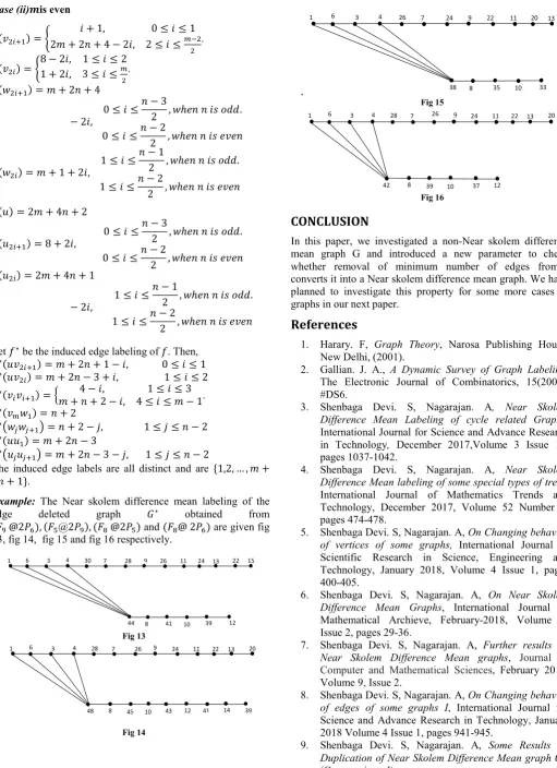
Example: The Near skolem difference mean labeling of the
edge deleted graph ∗ obtained from
( @2 ), ( @2 ), ( @2 ) and ( @ 2 ) are given fig
13, fig 14, fig 15 and fig 16 respectively.
CONCLUSION
In this paper, we investigated a non-Near skolem difference mean graph G and introduced a new parameter to check whether removal of minimum number of edges from converts it into a Near skolem difference mean graph. We have planned to investigate this property for some more cases of graphs in our next paper.
References
1. Harary. F, Graph Theory, Narosa Publishing House, New Delhi, (2001).
2. Gallian. J. A., A Dynamic Survey of Graph Labeling, The Electronic Journal of Combinatorics, 15(2008), #DS6.
3. Shenbaga Devi. S, Nagarajan. A, Near Skolem Difference Mean Labeling of cycle related Graphs, International Journal for Science and Advance Research in Technology, December 2017,Volume 3 Issue 12, pages 1037-1042.
4. Shenbaga Devi. S, Nagarajan. A, Near Skolem Difference Mean labeling of some special types of trees, International Journal of Mathematics Trends and Technology, December 2017, Volume 52 Number 7, pages 474-478.
5. Shenbaga Devi. S, Nagarajan. A, On Changing behavior of vertices of some graphs, International Journal of Scientific Research in Science, Engineering and Technology, January 2018, Volume 4 Issue 1, pages 400-405.
6. Shenbaga Devi. S, Nagarajan. A, On Near Skolem Difference Mean Graphs, International Journal of Mathematical Archieve, February-2018, Volume 9, Issue 2, pages 29-36.
7. Shenbaga Devi. S, Nagarajan. A, Further results on Near Skolem Difference Mean graphs, Journal of Computer and Mathematical Sciences, February 2018, Volume 9, Issue 2.
8. Shenbaga Devi. S, Nagarajan. A, On Changing behavior of edges of some graphs I, International Journal for Science and Advance Research in Technology, January 2018 Volume 4 Issue 1, pages 941-945.
9. Shenbaga Devi. S, Nagarajan. A, Some Results on Duplication of Near Skolem Difference Mean graph . (Communicated)
Fig 13
Fig 14
1 6 3 4 30 7 28 9 26 11 24 13 22 15
44 8 41 10 39 12
26
45
48 8
1 6 3 4 28 7 9 24 11 22 13 20
10 43 12 41 14 39
.
Fig 15
Fig 16
1 6 3 4 26 7 24 9 22 11 20 13
38 8 35 10 33
26
39
42 8
1 6 3 4 28 7 9 24 11 22 13 20
10. Shenbaga Devi. S, Nagarajan. A, Near Skolem Difference Mean Labeling of some Subdivided graphs. (Communicated)
11. Shenbaga Devi. S, Nagarajan. A, On Duplication of Near Skolem Difference Mean graph . (Communicated)
*******