Thermal Simulation of Solidification Process in Continuous Casting

Please cite this article as: A. Jabari Moghadam, H. Hosseinzadeh, Thermal Simulation of Solidification Process in Continuous Casting, International Journal of Engineering (IJE), TRANSACTIONS B: Applications Vol. 28, No. 5, (May 2015) 812-821

International Journal of Engineering

J o u r n a l H o m e p a g e : w w w . i j e . i r

Thermal Simulation of Solidification Process in Continuous Casting

A. Jabari Moghadam*, H. Hosseinzadeh

Department of Mechanical Engineering, Shahrood University of Technology, Post Box 316, Shahrood, Iran

P A P E R I N F O

Paper history: Received 31 August 2014

Accepted in revised form 30 April 2015

Keywords:

Heat Transfer Continuous Casting Stefan Condition Casting Speed

Boundary Immobilization Method Front-Fixing Method

A B S T R A C T

In this study, a mathematical model is introduced to simulate the coupled heat transfer equation and Stefan condition occurring in moving boundary problems such as the solidification process in the continuous casting machines. In the continuous casting process, there exists a two-phase Stefan problem with moving boundary. The control-volume finite difference approach together with the boundary immobilization method is selected to predict the position of moving interface and the temperature distribution. The approach is validated by some available models and the agreement is found to be satisfactory. Effects of the governing parameters such as Stefan number and casting speed on the evolution of the freezing front and temperature distributions are investigated. It is found that the variation of Stefan number has a strong influence on the growth of the shell thickness and the temperature distributions. For the same values of heat transferred from the mold, increasing Stefan number has significant results such as: accelerating the solidification process and increasing the solid thickness, enhancing the local heat flux in the liquid, and broadening the liquid zone affected by the cooling water jacket. As the casting speed becomes higher, the molten flow leaves the mold faster and the solid thickness entering the secondary cooling stage is decreased; meanwhile, the central liquid region has less time to be affected by the cooling water. Reducing casting speed results in decreasing the solid temperature; in other words, the solid layer becomes cooler.

doi: 10.5829/idosi.ije.2015.28.05b.20

1. INTRODUCTION1

Continuous casting technology is immensely

influencing the steelmaking practice in the worldwide. Basic components of a continuous casting machine (CCM) are schematically shown in Figure 1. The productivity and quality of a continuous casting product depend mainly on process parameters, i.e. casting speed, casting temperature, steel composition, melt cleanliness, water flow rates in the different cooling zones, etc. In this process, there are moving boundary problems known as Stefan problems involving heat conduction in conjunction with change of phase. Since this class of problems requires solving heat equation in an unknown region which has also to be determined as part of the solution, they are inherently non-linear problems. Owing to nonlinearity of thermal energy balance at the 1 _{*Corresponding Author’s Email: alijabari.m@aol.com (A. Jabari} Moghadam)

interface as well as unknown location of the phase change interface, analytical solutions are difficult to obtain, while numerical solutions are common.

Several methods have been developed and successfully applied to solve the Stefan problem with various boundary and initial conditions such as variational iteration method by Slota and Zielonka [1], finite difference method by Savovic and Caldwell [2] to solve one-dimensional Stefan problem with periodic Dirichlet boundary condition, boundary immobilization or front-fixing finite difference method by Caldwell and Savović

[3], a Lagrangian finite difference method by Yigit [4]. The variable space grid method based on finite difference was applied by Savović and Caldwell [5] and Ismail [6]. An alternative fixed grid method was investigated by Verma et al. [7], and an automatic differentiation method was also applied by Asaithambi [8].

Figure 1. Continuous casting machine

Figure 2. Sectional views of continuous casting zones

Figure 3. Isotherms in a square mold

Many researchers employed various numerical techniques to solve temperature field and location of phase change interface in continuous casting process [9-13]. Janik and Dyja [9] presented a three-dimensional numerical analysis of temperature field inside the mold during continuous casting of low carbon steel. Zhang et al. [10] studied a finite point method to model metal solidification process in continuous casting. In his work, the enthalpy method was used to calculate latent heat and the corresponding iterative solution was also

introduced. Kandeil et al. [11] performed a numerical study on this process in a square mold with unsteady two-dimensional energy equation based on the ADI finite difference method to predict temperature field and shell profile in the solidified steel strand. Alizadeh et al. [12] developed a mathematical unsteady two dimensional heat conduction model in Cartesian

coordinate system for computing temperature

distribution and predicting solid thickness in the mold region. An analytical model for local heat flux density in the mold in continuous casting of steel was presented by Alizadeh et al. [13].

In the case of solidification in continuous casting process, the domain boundary is not known in advance. This means that the solution of such problems requires solving diffusion or heat conduction equation in an unknown region which has to be determined as part of the solution. In the literature, finite difference methods are used to solve moving boundaries.

The phase-transition region where solid and liquid coexist is called interface. Its thickness may vary from a few Angstroms to a few centimeters, and its microstructure may be very complex, depending on several factors (material itself, rate of cooling, temperature gradient in liquid, surface tension, etc.). For most pure materials solidifying under ordinary freezing conditions at a fixed T_f, the interface appears (locally) planar and of negligible thickness. Thus, it may be thought of as a "sharp front", a surface separating solid from liquid at temperature T . f In other cases, typically

resulting from super cooling, or presence of multiple components (e.g. in binary alloys), the phase transition region may have apparent thickness and is referred to as a "mushy zone". In this zone, instead of melting temperature line (Tf), we have solidus and liquidus

lines. This mushy zone exists here because we have binary alloys. In the current work, by choosing suitable polar coordinates shown in Figure 2, we are able to simplify the problem. This one-dimensional approach is valid, because of the symmetrical geometry; isotherms of the mold region are in square form (Figure 3), and the dependent variables can be expressed in one variable

( )r . The methods employed in this research are

front-fixing or Boundary Immobilization Method (BIM) for liquid region and variable space grid method for solidified shell. Front-fixing method is an alternative formulation to implicit front-tracking methods, in which, the moving front is fixed by a suitable transformation in space coordinates [14, 15].

Figure 4. Control volume elemental for liquid region

Because the solidified shell thickness is varying continuously, we use the variable space grid method (VSG) for this region [5, 18, 19]. Solutions reported in the literature used finite difference methods to solve moving boundary problems [20]. In this study, we assume that the column cross-section is square, in which, the molten metal is descending at a constant speed. Deformation is also neglected to which it is typically subjected when bent by rollers. It is assumed that the vertical heat conduction is negligible.

2. PROBLEM FORMULATION

The problem illustrated in Figure 4 is governed by the energy equation in the molten (liquid) zone, the energy equation in the solid zone, the equation of Stefan condition and the energy equation in the mold.

To model the problem, the following assumptions are considered:

1. In the liquid pool, convective heat transfer is neglected and only conduction is considered, 2. Constant latent heat (Lf),

3. Like classical Stefan problems, density changes due to melting and solidification are neglected (r_l =r_s =r),

4. Each phase has its distinctive properties, that is,

k

_l

¹

k

_s and

c

_l

¹

c

_s ,

5. Conduction in the longitudinal direction of the billet has been neglected,

6. The surface heat flux based on the analytical approach is performed by Alizadeh et al. [13] and is assumed varying in the longitudinal direction.

7. The effects of mushy zone may be ignored, since its thickness is very small.

2. 1. Liquid Zone Energy conservation for the element in Figure 4 implies that:

(1)

in out st

q -q =E&

Also we have:

(2)

in r q =q

(3)

r out r

q

q q dr

r

¶

= +

¶

(4)

(2 ) l

st l z

T

E c rdr dz U

z

r æ ¶ ö

= ´ _{ç ÷}

¶

è ø

&

(5)

(2 ) l

r l

T

q k rdz

r

¶ =

-¶

Substituting these into Equation (1) yields:

(6)

2

2l 1 l 1 z l l

T T _U T

r

r r a z

¶ ₊ ¶ ₌ æ ¶ ö

ç ÷

¶ ¶ è ¶ ø

For a uniform casting speed throughout the entire region of the steel bar, relation between the longitudinal direction z and time t for a slice of steel (to move a distance z in casting machine) becomes:

(7)

z

z U t=

So, Equation (6) may be written as:

(8)

( )

2

2 1 1 , 0

l l l

l

T T T

r t

r

r r a t z

¶ ₊ ¶ ₌ ¶ _{£ <}

¶ ¶ ¶

where, a_l=k_l rc_land z

( )

t is the phase boundary position, in which z

( )

0 =L.

The initial and boundary conditions are:

(9a)

( ,0)

l in

T r =T

(9b) ( ( ), )

l liq

T z t t =T

(9c) (0, ) 0

l

T t r

¶ ₌

¶

2.2. Stefan Condition (The Liquid-Solid Interface)

When heat of solidification is taken into account, the differential equation describing the moving boundary becomes (note that both sides are positive):

( ) ( )

s l

f l s

r t r t

T T

d

L k k

dt r z r z

z r

- +

= =

¶ ¶

æ ö

- _{ç ÷} =

-¶ ¶

è ø (10)

2. 3. Solid Region According to Figure 5a and similar to section 2. 1., we get the following energy equation for the solid zone:

2

2 1 1

s s s

z s

T T _U T

r

r r a z

¶ ₊ ¶ ₌ æ ¶ ö

ç ÷

¶ ¶ è ¶ ø (11)

(12)

( )

2

2 1 1 ,

s s s

s

T T T

t r L

r

r r a t z

¶ ₊ ¶ ₌ ¶ _{< £}

¶ ¶ ¶

Initial and boundary conditions are:

(13a)

( ,0)

s sol

T r =T

(13b)

( ( ), )

s sol

T z t t =T

(13c) ( )

l s

r L T

k q z

r ₌

¶ ₌

-¶

2. 3. Spatial Coordinate Transformation In general, Equations (8), (10) and (12) with respect to (9) and (13) should be numerically solved. Applying the following spatial coordinate transformation to the model, we can fix the moving interface r =z_{( )}t at

1

h= in the new coordinate system

( )

h,t :

(14a) ( )

r t

h z

=

(14b) liq

l

in liq

T T

T T

q =

-(14c) sol

s

in sol

T T

T T

q =

-Then Equations (8), (10) and (12) take the following forms in new coordinate system

( )

h,t :

2 2

2

1 _{, 0 1}

l l l

l l t

q hzz q z q _h

h h a h a

æ ö æ ö

ç ÷ ç ÷

ç ÷ _{è ø}

è ø

¶ _{+ +} ¶ ₌ ¶ _{£ <}

¶ ¶ ¶

&

(15)

1 1

l s in sol s

l s

l in liq

c T T

d Ste

dt h c T T h

q q

z

z a a

h ₌- h ₌+

¶ - ¶

- =

-¶ - ¶

æ æ öæ ö ö

ç ç ÷ç ÷ ÷

ç _{è øè ø} ÷

è ø (16)

2 2

2 1

, 1

s s s

s s

l t

q hzz q z q _h

h h a h a

æ ö æ ö

¶ _{+ +} ¶ ₌ ¶ _{< £}

ç ÷ ç ÷

¶ _{è ø}¶ _{è ø} ¶

&

(17)

where, Ste is the Stefan number defined by (Ste =c T_l( _in -T_liq) L_f ) and l =L z( )t .

Boundary conditions are:

(18a)

( ,0) 1

l

q h =

(18b) (1, ) 0

l t

q =

(18c) (0, ) 0

l _t

q h

¶ ₌

¶

for liquid, and:

(19a) ( , 0) 0

s

q h =

19b)

(1, ) 0

s t

q =

(19c)

1

( ) s ( )

s in sol

l

k T T q z

h

q

z h ₌

¶

- ´ =

-¶

for solid. At this stage, the following empirical relation is used [13]:

(20)

(

)

( ) .

1

az w w w

z aH

m

a c Q T e

q z z U t

P e

r

-´ D

= ´ =

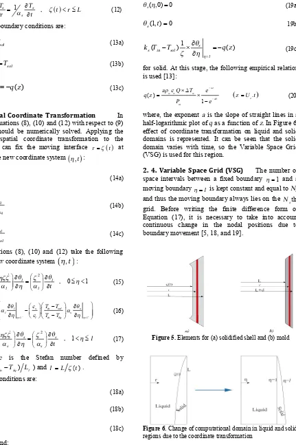
-where, the exponent a is the slope of straight lines in a half-logarithmic plot of q as a function of z. In Figure 6, effect of coordinate transformation on liquid and solid domains is represented. It can be seen that the solid domain varies with time, so the Variable Space Grid (VSG) is used for this region.

2. 4. Variable Space Grid (VSG) The number of space intervals between a fixed boundary h=1 and a moving boundary h=l is kept constant and equal to Ns,

and thus the moving boundary always lies on the N_sth

grid. Before writing the finite difference form of Equation (17), it is necessary to take into account continuous change in the nodal positions due to boundary movement [5, 18, and 19].

Figure 5. Elements for (a) solidified shell and (b) mold

Figure 6. Change of computational domain in liquid and solid

At the thi grid point, we have:

(21)

s s s

i

i t

t t t h

q q h q

h

¶ ¶ ¶ ¶

= ´ +

¶ ¶ ¶ ¶

And the node

h

_iis moved as follows:

(22) i

d dl

dt l dt

h h

= ´

in which the suffices t, i, and

h

are to be kept constant during differentiation. By substituting Equations (17) and (22) into (21), we have:

2

2 2

2 1

, 1

s i s s s

s s s

dl

l

t l dt

q h q q q

z z hzz

h

a a h h h a h

¶ ¶ ¶ ¶

= + + + < £

¶ ¶ ¶ ¶

æ ö

æ ö

æ

ö

ç ÷

ç ÷

ç

÷

è ø

è ø

è

ø

&

(23)

It should be noted that the grid size D =h 1 N_s varies with time as the interface moves, since the number of grid points is constant, and also_{dl dt = -Lz z}& 2

.

2. 5. Mold Region According to Figure 5b, the law of energy conservation in the mold implies that:

(24) 1

0 , L r L d m

r

r r r

q

¶ ¶

= £ £ +

¶ ¶

æ ö

ç ÷

è ø

in which:

(25) sol

m

in sol

T T

T T

q =

-subject to the following boundary conditions:

( ) ( , )

m L s L t

q =q (26a)

( ) m ( )

m in sol

r L d

k T T q z

r

q

= +

¶

- =

-¶ (26b)

Solution of Equation (24) subject to (26) is:

(27)

1ln 2

m C r C

q = +

where,

1

2

( ) ( )

( )

( ) ( )

( , ) ln

( )

m in sol

s

m in sol

q z L d

C

k T T

q z L d

C L t L

k T T

q

- ´ +

=

-´ +

= +

-(28)

3. FINITE DIFFERENCE METHOD

We employ an explicit finite difference method by using a forward difference scheme for the time derivative and

a central difference scheme for the space derivatives. Equation (15) becomes:

( )

, 1, , , , 1, 2 , , 1 , , 2

, 1, , 1,

2

1

2

l i m l i m l i m

l

l i m l i m

m _{l i m l i m}

i m m

i l

t

q q q

h a

q q

z _{h z z q q}

h a h

+

-+

+

-éæ _{- +} ö ù

êç_ç ÷_÷ ú

D

ê ú

D _{è ø}

= + _{ê ú}

-æ öæ ö

ê_{+ +} ú

ç ÷ç ÷

ê _{è D ø}ú

è ø

ë û

& (29)

where, q_{l i m, ,} ºq h_l

(

_i,t_m

)

. The quantities Dh and

D

t

are the constant space grid size and the time step, respectively. Equation (29) is used to obtain the temperature distribution at 0< <h 1; but for h=1, according to (18b), we have q_{l i m, ,} =0 in which i =N and m=1, 2, 3,…. For h=0, according to (15) and (18c), we use the following formula:

(

)

, 1, , ,

, , 1 , , 2 2

2 l l i m l i m

l i m l i m

m

ga q q

q q

z h

+ +

æ - ö

= + ç_ç ÷_÷

D

è ø (30)

It should be noted that at h=0, according to (18c), we haveq_{l i,-1,m} = q_{l i,+1,m}

(

i =1

)

.The Stefan condition (16) at h=1 _{in discretized form can be expressed as:}

, , , 1, , 2,

1

,1, ,2, ,3,

3 4

2

3 4

2

l N m l N m l N m

l

m m

m s m s m s m

s g Ste

M

q q q

a

h

z z

z q q q

a

h

-

-+

é æ - + ö ù

ê ç _D ÷ ú

´ ê è ø ú

= - _{ê ú}

- +

-æ ö

ê- _{ç ÷}ú

D

ê è øú

ë û

(31)

where, M =(c cs l) (

(

Tin-Tsol)

(

Tin-Tliq

)

)

. The following three-point backward and forward difference schemes are used for temperature gradients at the moving interface

(

h=1

)

[20]:

, , , 1, , 2, 2

1

3 4

( )

2

l N m l N m l N m

l _o

h

q q q

q

h

h h

-

-=

- +

¶

= + D

¶ D (32)

,1, ,2, ,3, 2

1

3 4

( )

2

s m s m s m

s _o

h

q q q

q _h

h ₌ h

- +

-¶ _{= + D}

¶ D (33)

The initial condition is z0=L. Finally, discretization

of Equation (23) yields:

( )

, 1, , , , 1,

, , 1 , , 2 2

, 1, , 1,

2 2

2

2

s i m s i m s i m

s

s i m s i m

m

s i m s i m

i m s i m

m i m m

t

L t

l

q q q

a

q q

z h

q q

h z a h z

z h z z h

+

-+

+

-æ - + ö

D

= + ç_ç ÷_÷

D

è ø

æ æ ö öæ - ö

+D ç_ç ç ÷+ + ÷_÷ç _D ÷

è ø

è ø

è ø

& & (34)

where, qs i m, , ºq hs

(

i,tm

)

. This formula is used to

obtain the temperature distribution at 1< <h l ; but for l

, , 1 , 1, 1 ( )

( )

s m

s l m s l m

s in sol

h

q z

k T T

z

q ₊ =q _{- +} - ´

- (35)

and for h=1, according to (19b), we have q_{s i m, ,} =0in which i=1 and m=1,2,3,….

TABLE 1. Input parameters of slab caster and

thermophysical properties of steel and cooling water Thermophysical properties of steel:

Solid Liquid

c (J kg-1o_C-1₎

ρ (kg m-3₎ k (W m-1o_C-1₎

Liquidus temperature (o_C) Solidus temperature (o_C) Lf (J kg-1)

Tin (oC) Ste

430 7400

33

1450 1425 260000

1530 0.25, 0.75, 1

825 7400

39

Geometry of the slab caster:

Section size (2L×2L) (m×m) H (m)

Uz (m min-1) d (m) k (W m-1o_C-1₎

0.28×0.28 0.67 0.6, 0.75, 0.9 0.02 315

Thermophysical properties of cooling water:

Q (l min-1₎

∆Tw (oC) c (J kg-1o_C-1₎

ρ (kg m-3₎ a (m-1₎

2347 5 4200 1000 1.25

Figure 7. Solidified shell thickness for Ste =0.1254

4. RESULTS AND DISSCUSION

Energy equations in liquid and solid zones as well as Stefan condition are solved using finite difference method. The values of thermo-physical properties and parameters used in the present work are summarized in Table 1 [13]. It is clear that liquid and solid temperatures, as well as Stefan condition (Equations (29), (31), (34)) are strongly coupled and need to be

solved simultaneously. The constant grid size for liquid region is h_l(º D =x 1N_l) (Nl =200is adopted).

At the beginning of the casting process, solidification does not occur; in fact, the molten metal is somewhat cooled and then solidification begins. Hence, for a short time after entering liquid in the mold, there is not any solid layer as well as the Stefan condition. Consequently, at this short time interval, only Equation (8) is satisfied and the liquid boundary condition at r =L becomes the liquid line temperature

( )

T_liq ; for each section of

z

, heat flow out from this boundary is equal to q z( ). Here, this time interval is considered 5Dt in which D =t

(

H U_z

)

100000 . The shell

thickness is initially very thin, so that the solution procedure is diverged; hence, for (l- <1) 0.01, we assume the solidified shell temperature is linear and for

(l-1)=0.01, we use Equation (34) in implicit form with 0.001

s

h = and for

(

l-1

)

>0.01, we use Equation (34). It is also assumed that the variable grid size is

(

1 10

)

s

h = l- (Ns =10is adopted) and the time step

(

)

g º Dt for all equations is D =t

(

H U_z

)

100000. In

Figure 7, the present computational values for the moving boundary position are plotted as a function of z. It can be seen that numerical values obtained for the position of the moving front are in agreement with available results from completely numerical solutions [13]. The Stefan number considered in [13] is

0.1254

Ste=

(

T_liq =1492,T_sol =1396

)

.

The key process parameters are Stefan number (Ste) and casting speed (Uz). Heat transferred to the cooling

water is assumed constant; and can be done practically by adjusting cooling water mass flow rate. Figure 8 illustrates variations of solid thickness for various values of Stefan number as well as casting speed (S =L-z ). Increasing Stefan number leads to increase in the solid thickness. Increase in Ste may be due to decrease in latent heat ( )Lf , and because heat exited

from the mold is the same for three cases, decreasing latent heat leads to accelerate the solidification process. Therefore, the solid thickness is increased. As can be seen from 8b, the thickness values are the same for three cases. This behavior is physically possible. Since with the assumption of equal exited heat values as well as invariant thermo-physical properties (including Stefan number), it is acceptable that the three thicknesses coincide. As the casting speed is increased, the molten flow leaves the mold faster and the solid thickness entering the secondary cooling stage will be decreased. As shown in Figure 9, an increase in the Stefan number results to accelerate solidification. As already mentioned, the solidification velocities for various

0 0.1 0.2 0.3 0.4 0.5 0.6 0.7

0 0.005 0.01 0.015 0.02

z(m )

S

h

e

ll

t

h

ic

k

n

e

ss

(

values of casting speed are the same, because the corresponding values of exited heat as well as other parameters are not changed.

(a)

(b)

Figure 8. Evolution of the moving boundary for: (a)

different Stefan number by constant casting speed

Uz=0.75(m min-1) and (b) different casting speed by

constant Stefan number Ste=0.25.

(a)

(b)

Figure 9. Velocity of the ζ for: (a) different Stefan number

by constant casting speed Uz=0.75(m min-1) as a function

of z and (b) different casting speed by constant Stefan number Ste=0.25 as a function of time.

(a) (b)

(c)

Figure 10. Temperature distribution in liquid region for

different Stefan numbers (a) Ste=0.25, (b) Ste=0.75 and (c)

Ste=1 for casting speed Uz=0.75.

(a) (b)

(c)

Figure 11. Temperature distribution in liquid region for

different casting speed (A) Uz=0.6, (B) Uz=0.75 and (C)

Uz=0.9 for Stefan number Ste=0.25.

Figure 10 represents temperature distributions in the liquid zone for various values of Stefan number. As Steincreases, a wider region of the liquid zone is affected by the cooling jacket; in fact, at higher Ste, more liquid becomes solid and less heat leaves for the cooling jacket due to solidification. On the other hand, as the values of heat exited from the mold are equal for the three cases, more heat leaves the liquid and so the affected region broadens. Temperature profiles in liquid for different values of casting speed are shown in Figure

0 0.1 0 .2 0.3 0 .4 0.5 0 .6 0 .7

0 0.01 0.02 0.03 0.04 0 .0 5

z( m )

S h el l th ic k n ess ( m) St e=0.25

St e=0 .75

St e=1

0 10 20 30 40 50 60 70

0 0 .0 05 0 .0 1 0.015 0 .0 2 0.025

ti m e ( s)

S h ell t h ic k n e ss (

m) t ime=53.6

ti me=44.66

Uz= 0 .6 (ti me=67)

Uz= 0 .75 (ti m e=53.6)

U_z= 0 .9 (ti me=44.66)

t ime=67

0 0 .1 0 .2 0 .3 0 .4 0.5 0 .6 0 .7

-2 -1.5 -1 -0 .5

0x 10

-3

z( m )

V el o ci ty o

f z

(

ms

-1)

St e=0 .25

St e=0 .75

St e=1

0 10 20 30 40 50 60 70

-6 -4 -2

0x 10

-4

ti m e ( s)

V e lo ci ty o

f z

(

ms

-1)

U_z=0.6

U_z=0.75

U_z=0.9

0.1 0.1 0.1 0.2 0.2 0.2 0.3 0.3 0.3 0.4 0.4 0.4 0.5 0.5 0.5 0.6 0.6 0.6 0.7 0.7 0.7 0.8 0.8 0.8 0.9 0.9 0.9 1 1 1 1 h z (m)

0 0.2 0.4 0.6 0.8 1

0 0.2 0.4 0.6 0.1 0.1 0.1 0.2 0.2 0.2 0.3 0.3 0.3 0.4 0.4 0.4 0.5 0.5 0.5 0.6 0.6 0.6 0.7 0.7 0.7 0.8 0.8 0.8 0.9 0.9 0.9 1 1 1 1 h z (m)

0 0.2 0 .4 0.6 0.8 1

0 0.1 0.2 0 .3 0.4 0 .5 0.6 0.1 0.1 0.1 0.2 0.2 0.2 0.3 0.3 0.3 0.4 0.4 0.4 0.5 0.5 0.5 0.6 0.6 0.6 0.7 0.7 0.7 0.8 0.8 0.8 0.9 0.9 0.9 1 1 1 1 h z (m)

0 0.2 0.4 0 .6 0.8 1

0 0 .1 0.2 0.3 0.4 0.5 0.6 0.1 0.1 0.1 0.2 0.2 0.2 0.3 0.3 0.3 0.4 0.4 0.4 0.5 0.5 0.5 0.6 0.6 0.6 0.7 0.7 0.7 0.8 0.8 0.8 0.9 0.9 0.9 1 1 1 1 h z( m)

0 0 .2 0.4 0.6 0 .8 1

0

0 .2

0 .4

0 .6 0.1

0.1 0.1 0.2 0.2 0.2 0.3 0.3 0.3 0.4 0.4 0.4 0.5 0.5 0.5 0.6 0.6 0.6 0.7 0.7 0.7 0.8 0.8 0.8 0.9 0.9 0.9 1 1 1 1 h z( m)

0 0.2 0.4 0.6 0.8 1

0 0.2 0.4 0.6 0.1 0.1 0.1 0.2 0.2 0.2 0.3 0.3 0.3 0.4 0.4 0.4 0.5 0.5 0.5 0.6 0.6 0.6 0.7 0.7 0.7 0.8 0.8 0.8 0.9 0.9 0.9 1 1 1 1 h z( m)

0 0.2 0.4 0.6 0.8 1

0

0.2

0.4

11. Decreasing casting speed causes the region affected by cooling water becomes wider and so more solid is formed.

(a)

(b)

(c)

Figure 12. Temperature distribution in solidified shell for

different Stefan numbers (a) Ste=0.25, (b) Ste=0.75 and (c)

Ste=1 for casting speed Uz=0.75.

(a)

(b)

(c)

Figure 13. Temperature distribution in solidified shell for

different casting speed (a) Uz=0.6, (b) Uz=0.75 and (c)

Uz=0.9 for Stefan number Ste=0.25.

Temperature distributions in solid layer for various values of Stefan number are shown in Figure 12. An increase in Stefan number leads to a decrease in the solid temperature. According to Equations (21) and (22), in which _{dl dt= -Lz z}& 2 _{, increasing Stefan} number results in decreasing z and increasing z&; hence, the right-hand side of Equation (21) and so

(

¶qs ¶t

)

i increase with negative sign. As shown in

Figure 13, reducing casting speed results in decreasing solid temperature (the solid layer becomes cooler). Figure 14 shows temperature distributions in the mold for different values of Stefan number and casting speed. According to Equations (27) and (28), and the fact that heat flux at each

z

is equal to q z

( )

, the only difference between these figures is due to the boundary condition (26a). In Figure 15, the r-direction heat flux exited from liquid at h=1 as a function of

z

is illustrated for various values of Steand U_z. Higher

Stefan number means lower latent heat, and so the heat exited from liquid is increased, since at each specified

z

, the total heat transfer to the cooling jacket are equal for every cases. Casting speed has a slightly effect on the heat flux, because according to Figure 9b, solidification velocities does not have significant difference and the total heat transfer rate is the same for the cases. Figure 16 illustrates local heat flux in liquid as a function of

h

at z =H for different values of Ste and U_z. Increasing Stefan number leads to increase

-1.5 -1 .35 -1_.3 5 -1.2 -1.2 -1_.05 -1.₀₅ -0 .9 -0.9 -0.9 -0_.75 -0_.75 -0.75 -0.6 -0.6 -0.6 -0 .45 -0_.45 -0.45 -0 .3 -0.3 -0.3 -0.3 -0 .15 -0_.15 -0.15 -0.15 h z( m) 1 l 0 0 .1 0 .2 0 .3 0 .4 0.5 0 .6 -1 .8 -1_.65 -1 .5 -1.5 -1_.35 -1_.35 -1.2 -1.2 -1 .05 -1_.05 -0.9 -0.9 -0.9 -0 .75 -0_.75 -0.75 -0 .6 -0.6 -0.6 -0 .45 -0_.45 -0.45 -0.45 -0 .3 -0.3 -0.3 -0.3 -0 .15 -0_.15 -0.15 -0.15 h z( m) 1 l 0 0 .1 0 .2 0 .3 0 .4 0 .5 0 .6 -1.8 -1 .65 -1_.65 -1 .5 -1.5 -1_.35 -1 .35 -1 .2 -1.2 -1 .05 -1_.05 -1.05 -0 .9 -0.9 -0.9 -0_.75 -0.₇₅ -0.75 -0 .6 -0.6 -0.6 -0.6 -0_.45 -0_.45 -0.45 -0.45 -0 .3 -0.3 -0.3 -0.3 -0 .15 -0 .15 -0.15

-0. 15 -0.15

local heat flux in liquid. Figure 16b shows that an increase in casting speed results in an increase in heat flux near the solid-liquid interface. However, this trend may be reversed for the smaller values of h. In fact,

increasing Uz which causes the central region has less

time to be affected by the cooling water. Therefore, the temperature gradients in this region will be smaller.

(a) (b)

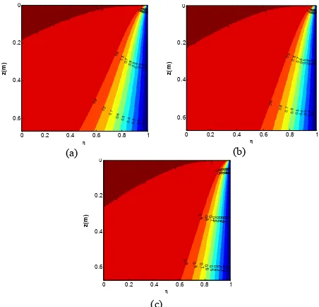
(c) (d)

Figure 14. Temperature distribution in mold region for

different values of Stefan number and casting speed (a)

Uz=0.75 & Ste=0.25, (b) Uz=0.75 & Ste=1, (c) Ste=0.25 &

Uz=0.6, (d) Ste=0.25 & Uz=0.9.

(a)

(b)

Figure 15. Local heat flux density as a function of z at

1

h

=

in liquid zone for: (a) different Stefan number by

constant casting speed Uz=0.75 (m min-1) and (b) different

casting speed by constant Stefan number Ste=0.75.

(a)

(b)

Figure 16. Local heat flux density as a function of

h

at

z=H in liquid zone for: (a) different Stefan number by

constant casting speed Uz=0.75 (m min-1) and (b) different

casting speed by constant Stefan number Ste=0.75.

5. CONCLUSION

In this research, solidification process and associated heat transfer in a square continuous casting mold are suitably modeled, and the governing equations are solved by a numerical scheme. It is evident that selecting this coordinate transformation simplifies the solution process, and therefore may be utilized for any similar cases. Two key parameters, namely Stefan number and casting speed, strongly affect the thermal characteristics of continuous casting. Provided that the magnitude of heat transfer (from mold to cooling water) remains constant, increasing Stefan number leads to accelerate solidification process and so to increase solid thickness. Higher Stefan number also results in broadening liquid zone affected by the cooling water jacket, and therefore enhancing local heat flux in it. A decrease in casting speed leads to a decrease in solid temperature. When casting speed is reduced, cooling effect of the water jacket diffuses more into the central region of the molten metal inside the mold, although this trend may be reversed for regions near the solid-liquid interface.

6. REFERENCES

1. Słota, D. and Zielonka, A., "A new application of he’s variational iteration method for the solution of the one-phase stefan problem", Computers and Mathematics with

Applications, Vol. 58, No. 11, (2009), 2489-2494.

2. Savović, S. and Caldwell, J., "Finite difference solution of one-dimensional stefan problem with periodic boundary conditions",

-2.6 -2.4 -2.4 -2 .2 -2.2 -2.2 -2 -2 -2 -1.8 -1.8 -1.8 -1.8 -1.6 -1.6 -1.6 -1.6 -1.4 -1.4 -1.4 -1.2 -1.2 -1.2 -1 -1 -1 -0.8 -0.8 -0.8 -0.6 -0.6 -0.4 -0.2

r (m )

z(

m)

0 .14 0 .15 0 .16

0 0 .1 0 .2 0 .3 0 .4 0 .5

0 .6 -2

.8 -2.8 -2.6 -2.6 -2 .4 -2.4 -2.4 -2.2 -2.2 -2.2 -2.2 -2 -2 -2 -2 -1.8 -1.8 -1.8 -1.6 -1.6 -1.6 -1.4 -1.4 -1.4 -1.2 -1.2 -1.2 -1 -1 -1 -0.8 -0.8 -0.6-0.4 -0.6

-0.2

r (m )

z(

m)

0 .14 0 .15 0 .16

0 0 .1 0 .2 0 .3 0 .4 0 .5 0 .6 -2.8 -2.6 -2.6 -2.4 -2.4 -2.4 -2.2 -2.2 -2.2 -2 -2 -2 -2 -1.8 -1.8 -1.8 -1.6 -1.6 -1.6 -1.4 -1.4 -1.4 -1.2 -1.2 -1.2 -1 -1 -1 -0.8 -0.8 -0.8 -0.6 -0.6 -0.4 -0.2

r ( m )

z(

m)

0 .14 0 .15 0 .16

0 0.1 0.2 0.3 0.4 0.5 0.6 -2.4 -2.2 -2.2 -2 -2 -2 -1.8 -1.8 -1.8 -1.6 -1.6 -1.6 -1.6 -1.4 -1.4 -1.4 -1.4 -1.2 -1.2 -1.2 -1 -1 -1 -0.8 -0.8 -0.8 -0.6 -0.6 -0.4 -0.2

r (m )

z(

m)

0 .14 0 .15 0 .16

0 0 .1 0 .2 0 .3 0 .4 0 .5 0 .6

0 0.1 0 .2 0 .3 0 .4 0.5 0 .6 0 .7

0 2 4 6

8x 10

5

z( m )

Lo c a l h ea t fl u x d e n si ty ( Wm -2) St e=0.25 St e=0.75 St e=1

0 0 .1 0 .2 0 .3 0 .4 0 .5 0 .6 0 .7

0 2 4 6

8x 10

5 z( m) L o ca l h ea t fl u x d e n si ty ( Wm -2)

Uz= 0 .6

U

z= 0 .75

U

z= 0 .9

0 0.2 0.4 0.6 0.8 1

0 1 2 3 4

5x 10

5 h L o c a l h e a t fl u x d e n si ty ( Wm -2 ) St e=0.25 St e=0.75 St e=1

0 0 .2 0 .4 0.6 0.8 1

0 0 .5 1 1.5

2x 10

5 h L o c a l h ea t fl u x d e n si ty ( Wm -2)

U_z=0 .6

U_z=0 .75

International Journal of Heat and Mass Transfer, Vol. 46, No. 15, (2003), 2911-2916.

3. Caldwell, J. and Savovic, S., "Numerical solution of stefan problem by variable space grid and boundary immobilization method", Journal of Mathematics Science, Vol. 13, (2002), 67-79.

4. Yigit, F., "One-dimensional solidification of pure materials with a time periodically oscillating temperature boundary condition",

Applied Mathematics and Computation, Vol. 217, No. 14,

(2011), 6541-6555.

5. Savović, S. and Caldwell, J., "Numerical solution of stefan problem with time-dependent boundary conditions by variable space grid method", Thermal Science, Vol. 13, No. 4, (2009), 165-174.

6. Ismail, K. and Henrıquez, J., "Solidification of pcm inside a spherical capsule", Energy Conversion and Management, Vol. 41, No. 2, (2000), 173-187.

7. Verma, A., Chandra, S. and Dhindaw, B., "An alternative fixed grid method for solution of the classical one-phase stefan problem", Applied Mathematics and Computation, Vol. 158, No. 2, (2004), 573-584.

8. Asaithambi, A., "Numerical solution of stefan problems using automatic differentiation", Applied Mathematics and

Computation, Vol. 189, No. 1, (2007), 943-948.

9. Janik, M. and Dyja, H., "Modelling of three-dimensional temperature field inside the mould during continuous casting of steel", Journal of Materials Processing Technology, Vol. 157, (2004), 177-182.

10. Zhang, L., Rong, Y.-M., Shen, H.-F. and Huang, T.-Y., "Solidification modeling in continuous casting by finite point method", Journal of Materials Processing Technology, Vol. 192, (2007), 511-517.

11. Kandeil, A., "Solidification of steel billets in continuous casting", (1991).

12. Alizadeh, M., Edris, H. and Shafyei, A., "Mathematical modeling of heat transfer for steel continuous casting process",

International Journal of ISSI, Vol. 3, No. 2, (2006), 7-16.

13. Alizadeh, M., Jahromi, A.J. and Abouali, O., "New analytical model for local heat flux density in the mold in continuous casting of steel", Computational Materials Science, Vol. 44, No. 2, (2008), 807-812.

14. Caldwell, J.a.N., D.K.S., "Mathematical modelling", Kluwer Academic Publishers, Dordrecht, (2004).

15. Vitorino, N., Abrantes, J. and Frade, J., "Numerical solutions for mixed controlled solidification of phase change materials",

International Journal of Heat and Mass Transfer, Vol. 53,

No. 23, (2010), 5335-5342.

16. Constales, D. and Van Keer, R., "Finite-element solutions for a direct problem in continuous casting and for its inverse", in International conference on computational modelling of free and moving boundaries. (1997), 97-102.

17. Caldwell, J. and Kwan, Y., "Spherical solidification by the enthalpy method and heat balance integral method", Advanced

Computational Methods in Heat Transfer VII, Vol., No.,

(2002), 165-174.

18. Kutluay, S., "Numerical schemes for one-dimensional stefan-like problems with a forcing term", Applied Mathematics and

Computation, Vol. 168, No. 2, (2005), 1159-1168.

19. Sadoun, N., Si-Ahmed, E.-K., Colinet, P. and Legrand, J., "On the boundary immobilization and variable space grid methods for transient heat conduction problems with phase change: Discussion and refinement", Comptes Rendus Mécanique, Vol. 340, No. 7, (2012), 501-511.

20. Anderson, J.D. and Wendt, J., "Computational fluid dynamics, Springer, Vol. 206, (1995).

Thermal Simulation of Solidification Process in Continuous Casting

A. Jabari Moghadam, H. Hosseinzadeh

Department of Mechanical Engineering, Shahrood University of Technology, Post Box 316, Shahrood, Iran

P A P E R I N F O

Paper history: Received 31 August 2014

Accepted in revised form 30 April 2015

Keywords:

Heat Transfer Continuous Casting Stefan Condition Casting Speed

Boundary Immobilization Method Front-Fixing Method

هﺪﯿﮑﭼ

ﻪﯿﺒﺷياﺮﺑﯽﺿﺎﯾرلﺪﻣ،ﻖﯿﻘﺤﺗﻦﯾارد

ﺪﻨﻧﺎﻣكﺮﺤﺘﻣزﺮﻣﺎﺑﻞﯾﺎﺴﻣردنﺎﻔﺘﺳاطﺮﺷوتراﺮﺣلﺎﻘﺘﻧاﻪﻟدﺎﻌﻣﻞﭘﻮﮐيزﺎﺳ

هﺎﮕﺘﺴﯾارددﺎﻤﺠﻧا ﺪﻨﯾآﺮﻓ

ﻪﺘﺨﯾريﺎﻫ

ﺖﺳاهﺪﺷﯽﻓﺮﻌﻣﻪﺘﺳﻮﯿﭘيﺮﮔ

.

ﻪﺘﺨﯾرﺪﻨﯾآﺮﻓرد

دﻮﺟويزﺎﻓودنﺎﻔﺘﺳاﻪﻟﺎﺴﻣ،يﺮﮔ

دراد

.

ﺎﺑ

ﻦﮐﺎﺳشورهاﺮﻤﻫﻪﺑلﺮﺘﻨﮐﻢﺠﺣدوﺪﺤﻣﻞﺿﺎﻔﺗدﺮﮑﯾورﺶﻨﯾﺰﮔ

ﺎﻣدﻊﯾزﻮﺗوكﺮﺤﺘﻣزﺮﻣﺖﯿﻌﻗﻮﻣ،زﺮﻣيزﺎﺳ

ﯽﻣﯽﻨﯿﺑﺶﯿﭘ

دﻮﺷ

.

لﺪﻣﯽﺧﺮﺑﺎﺑدﺮﮑﯾورﻦﯾارﺎﺒﺘﻋا

ﺖﺳاﺶﺨﺒﺘﯾﺎﺿر،دﻮﺟﻮﻣيﺎﻫ

.

ونﺎﻔﺘﺳادﺪﻋﺮﯿﻈﻧﻢﮐﺎﺣيﺎﻫﺮﺘﻣارﺎﭘﺮﺛا

ﻪﺘﺨﯾرﺖﻋﺮﺳ

ﺮﺑﺎﻣدﻊﯾزﻮﺗودﺎﻤﺠﻧاﻪﻬﺒﺟلﻮﺤﺗيورﺮﺑيﺮﮔ

ﯽﻣﯽﺳر

دﻮﺷ

.

ﺖﻣﺎﺨﺿﺪﺷرﺮﺑﯽﻓﺮﮕﺷﺮﺛانﺎﻔﺘﺳادﺪﻋﺮﯿﯿﻐﺗ

درادﺎﻣدﻞﯿﻓوﺮﭘوﻪﺘﺳﻮﭘ

.

ﻪﻈﺣﻼﻣﻞﺑﺎﻗﺞﯾﺎﺘﻧنﺎﻔﺘﺳادﺪﻋﺶﯾاﺰﻓا،ﺐﻟﺎﻗزاﻪﻠﻘﺘﻨﻣيﺎﻣﺮﮔنﺎﺴﮑﯾراﺪﻘﻣيازاﻪﺑ

زا،دراديا

ﻞﯿﺒﻗ

:

وﻊﯾﺎﻣردﯽﻌﺿﻮﻣﯽﯾﺎﻣﺮﮔرﺎﺷيﺎﻘﺗرا،ﺪﻣﺎﺟﺖﻣﺎﺨﺿﺶﯾاﺰﻓاودﺎﻤﺠﻧاﺪﻨﯾآﺮﻓﻪﺑنﺪﯿﺸﺨﺑبﺎﺘﺷ

ﻪﯿﺣﺎﻧشﺮﺘﺴﮔ

يا

ﮏﻨﺧبآﺖﮐاژزاﺮﺛﺎﺘﻣﻪﮐﻊﯾﺎﻣزا

ﺖﺳاهﺪﻨﻨﮐ

.

ﻪﺘﺨﯾرﺖﻋﺮﺳﻪﭽﻧﺎﻨﭼ

ﻊﯾﺮﺳباﺬﻣنﺎﯾﺮﺟ،دﻮﺷدﺎﯾزيﺮﮔ

كﺮﺗارﺐﻟﺎﻗﺮﺗ

ﯽﻣ

ﮏﻨﺧمودﻪﻠﺣﺮﻣﻪﺑهﺪﻧﻮﺷدراوﺪﻣﺎﺟﺖﻣﺎﺨﺿوﺪﻨﮐ

ﯽﻣﺶﻫﺎﮐيرﺎﮐ

يﺮﺘﻤﮐﺖﺻﺮﻓيﺰﮐﺮﻣﻊﯾﺎﻣﻪﯿﺣﺎﻧﻦﻤﺿرد؛ﺪﺑﺎﯾ

ﮏﻨﺧبآزايﺮﯾﺬﭘﺮﺛاياﺮﺑ

درادهﺪﻨﻨﮐ

.

ﻪﺘﺨﯾرﺖﻋﺮﺳﺶﻫﺎﮐ

ﯽﻣﺮﺠﻨﻣﺪﻣﺎﺟيﺎﻣدﺶﻫﺎﮐﻪﺑ،يﺮﮔ

ﻪﯾﻻ،ﺮﮕﯾدنﺎﯿﺑﻪﺑ؛دﻮﺷ

ﮏﻨﺧﺪﻣﺎﺟ

ﯽﻣﺮﺗ

دﻮﺷ