Please cite this article as: MS. Fallahnezhad, MS.Sajjadieh, P. Abdollahi, An Iterative Decision Rule to Minimize Cost of Acceptance Sampling Plan in Machine Replacement Problem. International Journal of Engineering (IJE) Transactions A: Basics, Vol. 27, No. 7, (2014): 1099-1106
International Journal of Engineering
J o u r n a l H o m e p a g e : w w w . i j e . i r
An Iterative Decision Rule to Minimize Cost of Acceptance Sampling Plan in
Machine Replacement Problem
MS. Fallahnezhad*a, MS.Sajjadiehb, P. Abdollahia
aIndustrial Engineering Department, University of Yazd, Yazd, Iran
bIndustrial Engineering Department, Amirkabir University of Technology, Tehran, Iran
P A P E R I N F O
Paper history:
Received 14 September 2013
Received in revised form 05 January 2014 Accepted 21 January 2014
Keywords:
Machine Replacement Acceptance Sampling Plan Control Threshold Policy Dynamic Programming
A B S T R A C T
In this paper, an optimal iterative decision rule for minimizing total cost in designing a sampling plan for machine replacement problem is presented using the approach of dynamic programming and Bayesian inferences. Cost of replacing the machine and cost of produced defectives have been considered in model. Concept of control threshold policy has been applied for decision making. If the probability of producing a defective was more than a control threshold then the machine is replaced otherwise its performenace will be accepted and continues its production. A numerical example along with sensitivity analysis is performed to show the application of proposed methodology.
doi: 10.5829/idosi.ije.2014.27.07a.11
1. INTRODUCTION 1
Machine replacement problem is an important topic in maintenance problems which can considerably influence on profit of companies. Many optimization models based on cost objective function are developed for machine replacement problem but not considering quality of items produced by machine in such models can lead to wrong decisions. Decision making about quality of machine based on inspecting the produced items usually results in application of sampling methods. Two approaches are often used to design an acceptance sampling design. First one is to design a sampling system which fulfills the constraints of first and second and type errors. For example, Aslam et al. proposed a new sampling system based on the constraints of first and second and type errors [1]. In addition, Chun and Rinks assumed the Beta distribution for proportion defective and they modified producer and consumer risks based on Bayes producer and consumer risks [2]. Fallahnezhad et al. presented a model of Markov chain approach in acceptance sampling plans
*Corresponding Author Email: [email protected] (MS. Fallahnezhad)
based on the cumulative sum of the number of successive conforming items [3]. Fallahnezhad analyzed the acceptance sampling design by using minimum angle method [4]. Aslam et al. proposed repetitive acceptance sampling plan with new decision rule [5]. The other approach is to design a sampling system which minimizes the total cost of decision making. Niaki and Fallahnezhad proposed a stochastic dynamic programming and Bayesian inferences concept to design an optimum sampling plan [6]. Fallahnezhad and Niaki proposed an economically optimal acceptance sampling policy based on number of successive conforming items [7]. Fallahnezhad and Hosseininasab proposed a single stage acceptance sampling plan by minimizing total cost of the system [8]. Fallahnezhad et al. proposed Bayesian acceptance sampling plan based on cost objective function [9].
used as an optimization technique in many industrial applications. Atkeson et al. had described a Random sampling plan based on Dynamic Programming for solving robot problem [10]. Furthermore, the Bayesian approach is used in order to design a sequential sampling system where the parameters of the model are updated in each stage. Chun and Sumichrast proposed Bayesian inspection models for certain item with some prior knowledge about the number of defects [11]. The inspection error is not considered in this model. Kotz and Johnson have considered a number of distributions arising from inspection sampling, when inspection error exists [12].
Many approaches have been proposed for the problem of machine replacement but analyzing the machine based on quality of produced items is not widely addressed [13]. In a paper, Fallahnezhad and Niaki employed control threshold policy and dynamic programming approach to design a decision-making framework in production environment. However, they did not consider the state of machine in next decision making stages after the decisions of accepting or replacing the machine [13]. Fallahnezhad proposed a dynamic programming approach for production and repair decisions. The state variable in his model was the rate of producing defectives. In addition, since his dynamic model was complicated, he could not obtain the optimal policy and he solved his model numerically [14]. In this research, it is tried to develop a cost optimal sampling plan for machine replacement problem subject to the constraints for first and second type errors that are basic concepts in acceptance sampling models. Analyzing quality of produced items in machine replacement problem usually leads to application of sampling plans approach. Two concepts which usually used in designing sampling plans are first and second type errors. In machine replacement problem, first type error is classifying a good machine as bad one and second type error is classifying a bad machine as good one. Therefore, the inspector may replace some good machines and accepts other bad machines. The classification of the machine to good or bad is based on the quality of produced items. The proportion of defectives produced by a good machine is less than acceptable quality level and the proportion of defectives produced by a bad machine is more than the limiting quality level.
The objective of this paper is to design a decision making framework for finite-horizon production and replacement problem. The rest of the paper is organized as follows. The problem statement and the presented model are in section 2. The solution algorithm along with numerical demonstration on the application of the proposed methodology comes in section 3 and a sensitivity analysis of proposed methodology comes in section 4. We conclude the paper in section 5.
2. THE MODEL
The dynamic programming is most applied technique to optimize multi stage decision-making problems [15]. Following definitions and notations are used in rest of the paper.
2. 1. Notations and Definitions Variable
p
is selected as the state variable of the system that is the: probability of producing a defective. Referring to Jeffrey’s prior [16], for the defective proportionp
, a Beta prior distribution with parameters 0.5 and 0.5 is considered. Using of the Bayesian inference, one can easily show that the posterior probability density function ofp
is,0.5
0.5
( 1)
( )
( 0.5) ( 0.5) (1 ) ,
n n
n n
f p p
p
a
b
a b
a b
-G + + =
G + G +
-(1)
where,an is the number of defectives and bn is the number of conforming items when
n
decision making stages are remained.Other parameters and notations of the model are as follows:
N
: The total number of items produced by the machinein each stage.
R: The cost of replacing the machine. C: The cost of having one defective.
( )
n
V p : Total cost associated with
p
when there aren
remaining stages to make the decision.n
d :The threshold for
p
. If the probability of producing a defective is more thandn, then machine is replaced otherwise the machine continues to produce items.AQL:Acceptable quality level.
LQL: Limiting quality level.
1
e
:The size of first type error probability in making a decision.2
e
:The size of second type error probability in making a decision.n
m
:The number of inspected items whenn
stages are remained.decision. One of these researches is a new approach in probability distribution fitting of a given statistical data that Eshragh and Modarres named it Decision on Belief (DOB) [17]. In this decision-making method, a sequential analysis approach is employed to find the best underlying probability distribution of the observed data.
It is tried to present a model for acceptance sampling plan by considering any stage of problem as a dynamic programming problem. It is assumed that ( ) n decision making stages exist and the objective is to obtain optimal policy for each stage. A sample from machine is taken and appropriate decision is selected based on obtained information from sample. In this policy, after determining the optimal decision for stage ( ) n based on the stages 1 ... ( -1) n then we move to s( -1) n stage
( -1) n . The same approach will be applied in stage
( -1) n so that a sample is gathered and the state variable of the system is determined then based on the cost in stages 1 ... ( - 2), n the optimal policy for stage ( -1) n is determined and so on. Decisions are as follows:
1- Accept the machine and continue the production in current stage
2- Replace the machine in current stage and continue to the next stage.
The proportion of defectives produced by machine is selected as state variable of the model. Its value is not known and it is tired to obtain its probability distribution by gathering data from machine. Niaki and Fallahnezhad [6], used Bayesian inference in their model to obtain a Beta distribution with parameters
,
n n
a b for proportion of defectives produced by machine. In this article, Bayesian concept is used to determine the probability distribution function of the defective proportion ( )p modeled as a Beta distribution with parameters an+0.5 , bn+0.5
[18]. Therefore, the probability of replacing a machine is (P p d³ n) and probability of accepting a machine is P p( £dn)where
n
d is the threshold for accepting or replacing the machine. ( ) n is defined as the number of decision-making stages remained and ( )p as state variable which denotes the probability of producing defectives then
( )
(
R+lVn-1 p1)
is the expected cost of machinereplacement whereR is the cost of replacing the machine in the current stage andlVn-1
( )
p1 is the cost ofnext stage when the machine is replaced where
p
1 is the probability of producing defective by a new machine. Also,(
CNE p p d(
< n)
+lVn-1( )
gp)
shows the expected cost of continuing the production processwhen the machine is accepted. Since E p p
(
<dn)
is theconditional expectation of probability of producing a defective by an accepted machine, thus
(
)
n CNE p p<d shows the cost of produced defective items. lVn-1
( )
gp represents the cost of next stage when the decision of continuing the production is chosen whereg>1is the degradation coefficient of machine state in each stage of production. In the other words, if the decision of continuing the production is selected, then proportion of defectives increases togpandl
is the discount factor for evaluating the cost of the next stage in the current stage (according to the approach of stochastic dynamic programming) . Thus, the stochastic dynamic equation for total cost of the system is defined as,( )
(
)
( )(
)
( )cos cos Reject Reject
cos Accept Accept .
E t E t P
E t P
=
+ (2)
Therefore, cost objective function is determined as follows:
( )
{
(
( ))
( )}
(
)
( )(
)
( ){
}
1 1
1 .
n n n
n n n
V p R V p P p d CNE p p d V p P p d
l
l g
-= + ³ +
< + < (3)
Equation (3) is the optimality equation which must be minimized to optimize the total cost of production environment.
( ) ( )
n n
n
H p MinV p
d
= (4)
machine is acceptable and second type error is the probability of accepting the machine when the proportion of defectives produced by machine is not acceptable. Then, in one hand ifp=AQL, the probability of replacing the machine will be smaller than
e
1 and in the other hand, in cases wherep LQL= , the probability of accepting the machine will be smaller thane
2[19]. A heuristic approach is used to apply the concepts of first and second type error in the model. First, it is assumed that the expected proportion of defectives produced by machine is equal toAQL( ) '
' + '
E p a AQL
a b
æ = = ö
ç ÷
è ø
also second one can use this fact
that the number of gathered samples is fixed
(
a' + 'b =mn)
. It is obvious that a b' , ' are different from
,
n n
a b that are obtained using sample information. The values a b' , ' are the number of defective and
non-defectives, respectively that are expected to be sampled from a lot produced by an acceptable machine. Now, one will be able to determine the parameters of Beta distribution for a proportion of defective items produced by an acceptable machine as follows:
( ) ( ) ' ' ' + ' . ' 1 ' + ' n n n AQLm
E p AQL
AQL m m a a a b b a b
ì = = ì =
ï Þï
í í =
-ïî
ï =
î
(5)
And the probability of replacing the machine is obtained by:
(
)
(
)
(
) (
)
( ) ( )( )( )
( )
11 1 1
1 1
1 1
(1 )
1
' 1 ' .
n n n n n n n n d
A Q L m A Q L m
p n
d
P p d
m
A Q L m A Q L m
p p
f p d p F d
e e e - - -³ = G ´
G G
-- £ ® £ ® - £
ò
ò
(6) 1t
is defined as lower boundary limit of dn, since( )
'
p n
F d is an increasing function of dn and
( )
1' 1
p n
F d ³ -e , thus:
(
)
' 1
1 1
1 .
n p
d ³F - -e =t (7)
First, it is assumed that the expected proportion of defectives produced by machine is equal toLQL
( )
'''' + ''
E p a LQL
a b
æ ö
= =
ç ÷
è ø
. The values a b'' , '' are the
number of defective and non-defectives that are expected to be sampled from a lot produced by an unacceptable machine, respectively. Therefore, when
( )
E p =LQL, following is obtained:
( )
(
)
" "
" + " .
" 1 " + "
n
n n
LQLm
E p LQL
LQL m m a a a b b a b
ì = = ì =
ï Þï
í í =
-ïî
ï =
î
(8)
The probability of accepting the machine is obtained as:
(
)
(
) (
( )
)
( ) ( )( )
0
1 1 1
2 (1 ) 1 n n n d n n n n
LQL m LQL m
m
P p d
LQLm LQL m
p - p - - e
G
£ = ´
G G
-- £ ®
ò
( )
2 2
0
"( ) " .
n
d
p n
f p £e ®F d £e
ò
(9)
If
t
2is defined as an upper boundary limit ofdnsince( )
"
p n
F d is an increasing function of dnand Fp"( )dn £e2,
thus:
( )
" 1
2 2.
n p
d £F- e =t (10)
Now, the Theorem 1 is used to determine the optimal value of control threshold
d
n.2. 3. Theorem 1 The optimal value of
d
n inEquation (3) is in one of these points, dn =t1 or
2
n
d
=t
or 1( )
1 1( )
3
n n
n
R V p V p
d t
CN
l - l - g
+
-= = . The
point t3can be optimal if its value was within the
boundary limits
(
t t1,2)
. The optimal value of dnis thepoint which minimizes the total cost of the system. The proof is given in Appendix A.
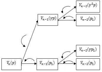
As can be seen in flowchart (Figure 1), the solution algorithm of the proposed approach is like a decision tree. As performed in decision trees, it starts from terminal nodes and using recursive approach; a decision is made in initial node. In this approach, first the value of V0(.) is obtained then using V0(.) values, the value of
V
1(.)are obtained Continuing this recursive approach, one can determine the values of V pn( ) . After obtaining the optimal value of V pn( ), the optimal value of control threshold will be determined. The suitable decision is made by comparing the mean value of proportion defective produced by the machine and the control threshold while if the mean value of Beta distribution obtained from sampled data was more than the control threshold then the machine is replaced otherwise it will continue its production in the next decision making stage.Figure 1. The iterative approach of proposed model
3. NUMERICAL EXAMPLE
To illustrate the application of the proposed model in designing a single machine replacement strategy, a numerical example with two stages is solved. Assume that (n =2) decision making stages are remained. Assume that five items have been produced
(
m2=5)
so that one of them has been defective ( )2 1, 2 4
a = b = .
Therefore, using the probability distribution defined in Equation (1), it is concluded that expected mean of the probability of producing a defective is as follows:
2 2 2
0.5 0.25 1
a
a b
+ =
+ + (11)
Assume that the cost of replacing machine is
R
=100$. In addition, a lot of N =100 items are produced in each stage. Assume that proportion of defectives produced by new machine is p1=0.05 and cost of producing each defective item is C =1$. The value of degradation coefficient is determined equal to g =1.1 and the discount factor is equal to l =0.9. Other parameters of sampling system are as follows:1 2
0 .1, 0.4, 0.2, 0.4
AQ L= LQ L= e = e =
By considering these parameter, to indicating total cost of machine replacement strategy, first it is needed to evaluate the function V0(.) (the state is
p
and stage is0
n = , it represents the cost at the end of decision making process) that is assumed as follows:
0( ) 1000
V p = p (12)
It is obvious that cost of machine maintenance at last decision making stage is an increasing function of machine state and to evaluate its value, one can use linear or non-linear regression for historical data. It means that a database containing the state of the machine and its corresponding maintenance cost at the end of decision making horizon is gathered from past
data and then one can fit the best regression model to data using available software. Using Equation (3) following is obtained,
( )
{
(
( ))
( )}
(
)
( )(
)
( ){
2 2 1 1 2 2}
0.2 5 0 .0 5
0.9 0.2 75 .
V R V P p d
C N E p p d V P p d
l
= + ³ +
< + < (13)
To evaluate above function, first it is needed to determine V1
(
0.05)
and V1(
0.275)
that are obtained asfollows:
3. 1. First Step The value of V1
(
0.05)
isdetermined as follows:
( )
{
(
( ))
( )}
(
)
( )(
)
( ){
1 1 0 0 1 1}
0 .0 5 0 .0 5
0.9 0 .0 5 5 .
V R V P p d
C N E p p d V P p d
l
= + ³ +
< + < (14)
To evaluate above function again the probability density function of probability of producing a defective item by a machine is needed where the state variable of machine is 0.05. Assume the function f p( )is such probability density function. To obtainf p( ), the heuristic approach explained in the last section for obtaining boundary limit is used thusf p
( )
is a Beta density function with parametersa b, that are determined using following equations,( )
0.05, 2 5.E p m
a a b
a b+ = = + = = (15)
After obtaining f p
( )
, first the possible values of thresholds should be obtained in order to determine the optimal value ofd
1 by substituting these three possiblevalues 1 1 1 2
(
)
(
)
0 0
1
, ,
0.05 0.055
d t d t
R V V
d
CN
l l
= =
æ ö
ç + - ÷
ç = ÷
ç ÷
è ø
in objective
functions and selecting one that minimizes the objective function. The values t1=0.17 and t2=0.33 are obtained using Equations (7) and (10). Moreover, the value t=0.955 is obtained with considering Equation (11). Since the value of t3 =0.955 is not within
(
t t1, 2)
thus this value for d1is not feasible and is ignored. After substituting the possible values for d1in objective function, we can determine the value of V1
(
0.05)
as denoted in Table 1. Then, it is seen that minimum occurs in and V1(
0.05)
=59.7.( )
{
(
( ))
( )}
(
)
( )(
)
( ){
}
1 0 1
1 0 1
0.275 0.0 5
0.9 0 .30 25 .
V R V P p d
C N E p p d V P p d
l
= + ³ +
< + < (16)
To evaluate above function, it is needed to evaluate the probability density function of probability of producing a defective item by a machine where the state variable of machine is 0.275 . Assume f p( )is such probability density function thus similar to Equation (15), f p
( )
is a Beta density function with parametersa b, that are determined using following equation,( ) 0.275, 2 5
E p m
a a b
a b+ = = + = = (17)
After obtaining f p
( )
, first the values of thresholds are obtained in order to determine the optimal value ofd1.These three possible values
( ) ( )
1 1 1 2
0 0
1 3
, ,
0.05 0.3025 d t d t
R V V
d t
CN
l l
= =
æ ö
ç + - ÷
ç = = ÷
ç ÷
è ø
are substituted in
objective functions and one that minimizes the objective function is selected. After determining the optimal value of d1, the value of V1(0.275) can be obtained. The
results are shown in Table 2. It is seen that minimum occurs in d1= =t1 0.17and V1
(
0.275)
=192.3. 3. Third Step. After determining the values
of V1
(
0.05)
and V1(
0.275)
, the value of V2(
0.25)
can beobtained as follows:
( )
{
(
( ))
( )}
(
)
( )(
)
( ){
2 2 1 1 2 2}
0.25 0.05
0.9 0.275 .
V R V P p d
CNE p p d V P p d
l
= + ³ +
< + < (18)
To evaluate above function, these three possible values
( ) ( )
2 1 2 2
1 1
2 3
, ,
0.05 0.275
d t d t
R V V
d t
CN
l l
= =
æ ö
ç + - ÷
ç = = ÷
ç ÷
è ø
are substituted in
objective functions and select one that minimizes the objective function. According to the results of steps 1 and 2, the optimal solution for V2(0.25) is obtained as shown in Table 3. It is clear, that minimum occurred in
2 1 0.17
d = =t and optimal value of system cost is 168. Now, since E p
( )
=0.25³d2= =t1 0.17; therefore, the machine should be replaced when two decision making stages are remained.
4. SENSITIVITY ANALYSIS
A sensitivity analysis is performed to analyze the effects of changing parameters on the optimal solution and
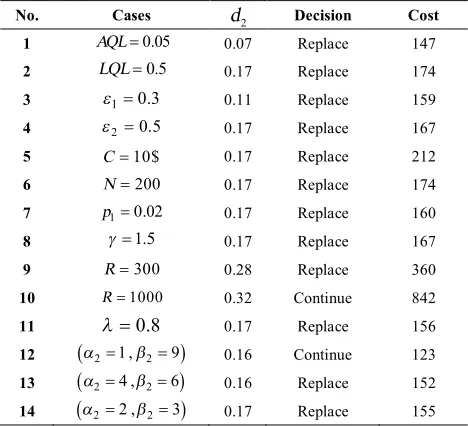
cost. All parameters were varied in this production system and their effects have been analyzed in this section. In each case of sensitivity analysis, one parameter of the model is varied in order to analyze its effects on the final solution of the model and verify its behavior. It is tried to adjust the parameter value in a level so that one can easily interpret their effects on the model. The results are shown in Table 4.
It is seen from case one that by decreasing
0.05
AQL= , the required quality for the production improves. Therefore, the optimal decision would still be replacing the machine again. This result is justified due to optimality of this decision in the case AQL=0.1. In the case two, it is seen that the optimal decision remains fixed again which implies that the risk of producer will be more important in this case.
TABLE 1. The values of V1(0.05)for two possible values of d1 1 0.17
t = t2=0.33
( )
1 0.05
V 59.7 68.43
TABLE 2. The values of V1
(
0.275)
for two possible values of d1 1 0.17t = t2=0.33 t3<0
( )
1 0.275
V 192 242 -
TABLE 3. The values of V2(0.25)for two possible values of d2
1 0.17
t = t2=0.33 t3<0
( ) 2 0.25
V 168 186 -
TABLE 4. The results of sensitivity analysis for the proposed sampling plan
No. Cases d2 Decision Cost
1 AQL=0.05 0.07 Replace 147
2 LQL=0.5 0.17 Replace 174
3 e1=0.3 0.11 Replace 159 4 e2=0.5 0.17 Replace 167 5 C=10$ 0.17 Replace 212
6 N=200 0.17 Replace 174
7 p1=0.02 0.17 Replace 160
8 g =1.5 0.17 Replace 167
9 R=300 0.28 Replace 360
10 R=1000 0.32 Continue 842
11 l=0.8 0.17 Replace 156
12 (a2=1 ,b2=9) 0.16 Continue 123
13 (a2=4 ,b2=6) 0.16 Replace 152
Since the producer wants to make a decision about its production; so, he mostly considers the risk of producer. It is concluded from case three that the optimal decision remains fixed by increasing the probability of first type error. This result is justified due to large value of proportion defective which results in defective production. Therefore, replacing the machine is needed even for larger values of first type error probability. It is concluded from case four that the optimal decision remains fixed by increasing the probability of second type error. Since the producer optimizes its cost, the probability of second type error that is risk of consumer has less importance in this case. It is seen from case five that the optimal decision remains fixed by increasing the cost of non-conforming items. Since the cost of continuing the production process increases in this case, the optimal decision does not change. It is obtained from case six that the optimal decision remains fixed by increasing the number of items in lot. Since the cost of continuing the production process increases in this case; so, the decision of replacing the machine will still remain optimal. It is obtained from case seven that the optimal decision remains fixed by decreasing the proportion defective of a new machine. Since the cost of replacing the machine decreases in this case, the decision of replacing the machine will still remain optimal. It is seen from case eight that the optimal decision remains fixed by increasing the degradation coefficient. Since the cost of continuing the production process increases in this case; therefore, the optimal decision does not change. It is concluded from case nine that the optimal decision does not change by increasing the replacement cost to
300
R = . This result is justified due to large value of proportion defective such that increasing replacement cost cannot change the optimal decision. However, it is seen form case ten that optimal decision will be to continue production process for sufficiently large values of replacement cost
(
R=1000)
. It is obtained in case eleven that decreasing the discount factor cannot change the optimal decision in this case but it reduces the total cost of the system that is reasonable. After improving the quality of production in case twelve, it is seen that the optimal decision is to continue the production as expected. The cases thirteen and fourteen confirm this result. In general, the results of sensitivity analysis verify the outcome of the proposed model in different conditions.5. CONCLUSION
In this article, a control threshold policy is applied to design an acceptance sampling system for one machine maintenance problem. This model proposes an optimal
iterative decision rule for minimizing total costin designing a sampling plan for machine replacement problem based on the methods of dynamic programming and Bayesian inferences. In order to determine the optimal policy, a cost objective function based on the cost of replacement and the cost of defectives is considered. The dynamic programming concept is used to consider the stochastic state of the machine in different stages. The optimal decision is determined based on the numerical methods. As shown in numerical example, the application of the model is quite simple and reasonable. The application of proposed model is justified in the production environments when machine deterioration can be monitored using the quality of produced items. The model can be extended to the cases that other decisions existed.
[1-19]
6. REFERENCES
1. Aslam, M., Fallahnezhad, M.S. and Azam, M., "Decision procedure for the weibull distribution based on run lengths of conforming items", Journal of Testing and Evaluation, Vol. 41, No. 5, (2013), 826-832.
2. Chun, Y.H. and Rinks, D.B., "Three types of producer's and consumer's risks in the single sampling plan", Journal of Quality Technology, Vol. 30, No. 3, (1998).
3. Niaki, A. and Nezhad, F., "A new markov chain based acceptance sampling policy via the minimum angle method",
Iranian Journal of Operations Research, Vol. 3, No. 1, (2012), 104-111.
4. Nezhad, M.S.F., Niaki, S.T.A. and Hossein, M., "A new acceptance sampling plan based on cumulative sums of conforming run-lengths", Journal of Industrial and systems engineering, Vol. 4, No. 4, (2011), 256-264.
5. Aslam, M., Niaki, S., Rasool, M. and Fallahnezhad, M., "Decision rule of repetitive acceptance sampling plans assuring percentile life", Scientia Iranica, Vol. 19, No. 3, (2012), 879-884.
6. Niaki, S.A. and Nezhad, M.F., "Designing an optimum acceptance sampling plan using bayesian inferences and a stochastic dynamic programming approach", Scientia Iranica Transaction E-Industrial Engineering, Vol. 16, No. 1, (2009), 19-25.
7. Nezhad, M.S.F. and Niaki, S.T.A., "A new acceptance sampling policy based on number of successive conforming items",
Communications in Statistics-Theory and Methods, Vol. 42, No. 8, (2013).
8. Nezhad, M.S.F. and Nasab, H.H., "Designing a single stage acceptance sampling plan based on the control threshold policy",
International Journal of Industrial Engineering, Vol. 22, No. 3, (2011), 143-150.
9. Fallahnezhad, M., Niaki, S. and Zad, M.V., "A new acceptance sampling design using bayesian modeling and backwards induction", International Journal of Engineering-Transactions C: Aspects, Vol. 25, No. 1, (2012), 45.
12. Kotz, S. and Johnson, N.L., "Effects of false and incomplete identification of defective items on the reliability of acceptance sampling", Operations Research, Vol. 32, No. 3, (1984), 575-583.
13. Nezhad, M.S.F. and Niaki, S.T.A., "A multi-stage two-machines replacement strategy using mixture models, bayesian inference, and stochastic dynamic programming", Communications in Statistics-Theory and Methods, Vol. 40, No. 4, (2011). 14. Fallahnezhad, M.S., "A finite horizon dynamic programming
model for production and repair decisions", Communications in Statistics-Theory and Methods, Vol., No. just-accepted, (2014), 00-00.
15. Ross, S.M., "Introduction to stochastic dynamic programming: Probability and mathematical, Academic Press, Inc., (1983). 16. Tang, B., Nair, V.N. and Xu, L.-a., "Bayesian inference for some
mixture problems in quality and reliability", Journal of Quality Technology, Vol. 33, (2001), 16-28.
17. Eshragh, A. and Modarres, M., "A new approach to distribution fitting: Decision on beliefs", Journal of Industrial and Systems Engineering, Vol. 3, No. 1, (2009), 56-71.
18. Fallahnezhad, M. and Fakhrzad, M., "Determining an economically optimal(n, c) design via using loss functions",
International Journal of Engineering, Vol. 25, No. 3, (2012), 197-201.
19. Montgomery, D.C., "Introduction to statistical quality control, John Wiley & Sons, (2007).
Appendix A. Method of obtaining the optimal threshold:
The first derivatives of
V p
n( )
is taken in Equation (3) with respect tod
nand set it equal to zero. That is,( ) 0. n n V p d ¶ = 
SinceP p( £dn)=F d( )n and
( ) ( ) ( ) 0 0 n n d n d
pf p dp E p p d
f p dp
< =
ò
ò
, thus following is obtained,
( )
{
( )}
( )
{
( )}
1 1
1 ( ) 0
0. n
n n
n
n n n
V p
f d R V p
d
f d CNd V p
l l g -¶ = ® - + + ¶ + = Therefore,
( )
( )
1 1 1
3 .
n n
n
R V p V p
d t
CN
l - l - g
+
-= -= (A1)
Since 2 ( )
2 ( ) 0 n n n n V d CNf d d
¶ = >
thus, it is insured that
( ) ( )
1 1 1
n n
n
R V p V p
d
CN
l - l - g
+
-= minimizes the objective
functions. Now, in the solution algorithm, three
possible values 1( )1 1( )
1, ,2 3
n n
n
R V p V p
d t t t
CN
l - l - g
+ -æ ö = ç ÷ è ø are
analyzed and one which minimizes the objective function V pn( )is selected.
An Iterative Decision Rule to Minimize Cost of Acceptance Sampling Plan in
Machine Replacement Problem
MS. Fallahnezhada, MS.Sajjadiehb, P. Abdollahia
aIndustrial Engineering Department, University of Yazd, Yazd, Iran
bIndustrial Engineering Department, Amirkabir University of Technology, Tehran, Iran
P A P E R I N F O
Paper history:
Received 14 September 2013
Received in revised form 05 January 2014 Accepted 21 January 2014
Keywords:
Machine Replacement Acceptance Sampling Plan Control Threshold Policy Dynamic Programming هﺪﯿﮑﭼ ارد ﯾ ﻦ ،ﻪﻟﺎﻘﻣ ﮏﯾ ﻤﺼﺗهﺪﻋﺎﻗ ﯿ ﻢ ﮔﯿ ﺮ ي ﻬﺑ ﯿ ﻪﻨ ﯽﺘﺸﮔزﺎﺑ اﺮﺑ ي
ﺰﻫنﺪﻧﺎﺳرﻞﻗاﺪﺣﻪﺑ
ﯾ ﻪﻨ
ﺣاﺮﻃردﻞﮐ
ﯽ ﯾ ﮏ
ﮔﻪﻧﻮﻤﻧحﺮﻃ
ﯿﺮ ي اﺮﺑ ﻪﻟﺎﺴﻣي ﻮﻌﺗ ﯾ ﺾ ﻪﻣﺎﻧﺮﺑشورزاهدﺎﻔﺘﺳاﺎﺑهﺎﮕﺘﺳد يﺰﯾر
ﻮﭘ ﯾﺎ ﺑجﺎﺘﻨﺘﺳاو ﯿﺰ ي ﺖﺳاهﺪﺷﻪﺋارا
. ﺰﻫ ﯾ ﻪﻨ ﺎﺟ ﯾ ﺰﮕ ﯾﻨ ﯽ ﺷﺎﻣ ﯿ ﻦ
ﺰﻫوتﻻآ
ﯾ ﻪﻨ ﺑاﺮﺧ ﯽ ﺎﻫ ي ﻟﻮﺗ ﯿﺪ ﺷ هﺪ
ﺖﺳاهﺪﺷﻪﺘﻓﺮﮔﺮﻈﻧردلﺪﻣردهﺎﮕﺘﺳدﻂﺳﻮﺗ
.
ﺳمﻮﻬﻔﻣ
ﯿ ﺖﺳﺎ اﺮﺑلﺮﺘﻨﮐﻪﻧﺎﺘﺳآ ي ﻤﺼﺗ ﯿ ﻢ ﮔﯿ ﺮ ي هدﺎﻔﺘﺳا ﺖﺳاهﺪﺷ .
ﻟﻮﺗلﺎﻤﺘﺣاﺮﮔا ﯿﺪ ﻌﻣ ﯿ بﻮ ﺑﯿ ﺶ لﺮﺘﻨﮐﻪﻧﺎﺘﺳآزا دﻮﺷ ﺎﺟهﺎﮕﺘﺳد ﯾ ﺰﮕ ﯾ ﻦ دﻮﺷﯽﻣ ﻏرد ﯿﺮ اﯾ ﻦ ترﻮﺻ ﺖﯿﻔﯿﮐ ﺬﭘنآ ﯾ ﻪﺘﻓﺮ ﻣ ﯽ ودﻮﺷ ﻪﺑ ﻟﻮﺗ ﯿﺪ ادا ﻣﻪﻣ ﯽ ﺪﻫد . ﯾ ﮏ دﺪﻋلﺎﺜﻣ ي ﺰﺠﺗﺎﺑهاﺮﻤﻫ ﯾﻪ و ﻠﺤﺗ ﯿ ﻞ ﺳﺎﺴﺣ ﯿ ﺖ هﻮﺤﻧ دﺮﮑﻠﻤﻋ ﭘشور ﯿ دﺎﻬﻨﺸ اري ﻣنﺎﺸﻧ ﯽ ﺪﻫد .