Image Zooming using Non-linear Partial Differential Equation

(1)

International Journal of Engineering

J o u r n a l H o m e p a g e : w w w . i j e . i r

Image Zooming using Non-linear Partial Differential Equation

N. Nowrozian * a_{, H. Hassanpour}b

a_{Department of Computer Engineering, Islamic Azad University Sari Branch, Sari, Iran} b_{Department of Computer Engineering, Shahrood University of Technology, Shahrood, Iran}

P A P E R I N F O

Paper history: Received 18 June 2013

Received in revised form 20 August 2013 Accepted 22 August 2013

Keywords:

Image Zooming

Partial Differential Equations (Pdes) Nonlinear Fourth-order PDE

Locally Adaptive Zooming Algorithm (LAZ) Unsharp Masking.

A B S T R A C T

The main issue in any image zooming techniques is to preserve the structure of the zoomed image. The zoomed image may suffer from the discontinuities in the soft regions and edges; it may contain artifacts, such as image blurring and blocky, and staircase effects. This paper presents a novel image zooming technique using Partial Differential Equations (PDEs). It combines a non-linear Fourth-order PDE method with the Locally Adaptive Zooming (LAZ) algorithm. The proposed method uses high-resolution image obtained from LAZ algorithm to construct zoomed image by Fourth-order PDE. This proposed method preserves edges and minimizes blurring and staircase effects in the zoomed image. In order to evaluate image quality obtained from the proposed method, this paper focuses on both subjective and objective assessments. The results of these measures on a variety of images show that the proposed method is superior over the other image zooming methods.

doi:10.5829/idosi.ije.2014.27.01a.03

1. INTRODUCTION1

Image zooming techniques plays an important role in the area of image processing and computer version. Most of the zooming algorithms use some image interpolation techniques. Image interpolation is to find a set of unknown pixel values from a set of known pixel values in an image.

Image zooming has many applications in fields such as medical imaging [1], electronic publishing, satellite images, images found on web [2-4], license plate identification or face recognition systems in legal procedures The main emphasis in many image zooming techniques is the edge sharpness (clarity) and being artifact-free (such as blurring and jagging and staircase effects).

Varieties of image zooming techniques exist. For instance, traditional image zooming techniques used to apply linear interpolation methods or non-adaptive methods to make the High-Resolution (HR) images. Common examples of the algorithm are the nearest neighbor [5], bicubic and sinc [6]. Nearest neighbor

*_{Corresponding Author Email:} _{[email protected]} _(N.

Nowrozian)

interpolation algorithm is used the nearest pixel for interpolation point. This method improves the processing speed. Bicubic takes neighbors 4 * 4 to calculate the interpolation point. Sinc uses a large number of pixels to find the value of interpolation point. Some other examples are Gaussian and varieties of Spline functions [7] and BILinear Interpolation (BILI) algorithm. In general, the basic problem of linear algorithms is blurring along the edges or artifacts around them. These technologies do not properly restore zooming images at the edges and areas with high contrast values. The issue is being unable linear technologies in transmission of the new information to the image. In contrast, the biggest advantage of linear models is their high speed in processing.

(2)

Zooming (AZ) algorithm [9], other examples are edge-directed algorithms in [10-12].

In recent years, methods based on Partial Differential Equations (PDEs) have been proposed and have shown better performance than the previous methods. One of the widely used techniques based on PDEs in image processing uses heat equation [13, 14]. In [1], the method is a combination of the Curvature-driven and Edge-stopping. The model protects small curves and large gradients. In addition, it has shown a satisfactory performance to maintain image edges. Curvature Interpolation Method (CIM) in [15] can be regarded as another example for zooming methods based on PDEs.

PDE-based methods have been widely used for image denoising. The images resulting from the application of these techniques enable to good smoothness images while preserve the edges sharpness. A fourth-order PDE is used as an effective method for noise removal. This method reduces the staircase effects considerably and textures are well preserved.

Based on these specifications, this paper has focused on a zooming method based on PDEs. The basic idea is introduce a fourth-order PDE to smooth the image and reduces the staircase effects.

The proposed method combines Fourth-order PDE method with LAZ algorithm. This technology can minimize artifacts and maintains the edges satisfactorily. In addition, our results verify the superiority of the proposed method compared to LAZ interpolation and some other zooming methods (include AZ, CIM, and BILI).

Next section briefly describes four methods for image zooming. The proposed method is introduced in Section 3. In Section 4, image quality assessment is presented. Experimental results and finally the conclusion are provided in Sections 5 and 6.

2. PRELIMINARIES

Here, we will describe four methods such as BILI, LAZ, AZ, and CIM for image zooming.

2. 1. Linear Algorithms

2. 1. 1. BILinear Interpolation The BILI algorithm in [5] uses the neighboring 2*2 to calculate unknown pixels. The value of unknown pixel find from weighted average of the four neighboring pixels. The advantage of this method is to create zoomed image of high quality and low processing time. However, this method is not suitable images that they are focused on the edge; it creates a continuous staircase effects over the edge. It also accompanies with blurring effects because of the use of a weighted average of neighboring pixels [6].

2. 2. Non-linear Algorithms

2. 2. 1. The Locally Adaptive Zooming Algorithm

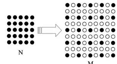
LAZ in [8] introduced using information about discontinuities (sharp luminance variations) by a non-linear iterative interpolation procedure for the image zooming. Thus, it doubles an LR image N with a size

(i*j) to a HR image M with size (2i-1, 2j-1). Therefore, we have: M (2i-1, 2j-1) =N (i, j) (Figure 1, the blank dots and the black dots, respectively, denote the pixels from M and unknown pixels). The next step is to considering two threshold values, and edges found in different directions.

Five directions based on different edge types, namely: uniformity, edge in the SW–NE direction, edge in the NW–SE direction, edge in the NS direction, and finally edge in the EW direction are considered.

All the pixels are scanned in M and the unknown pixels which are even in terms of the row and column coordinate and determined based on the average on either side of neighboring pixels (with regard to the direction of the edge obtained). (The gray dot labeled F shown in Figure 2(a)).

Then, in the same way, the unknown pixels with the least odd one row and column coordinate have been determined while considering the two conditions. (In Figure 2(b) and 2(c), the gray dot labeled R is unknown pixel). The two conditions to be considered are as follows: The first condition is that F1 and F2 are both unknown. The second condition assumes that F1 and F2 are both defined.

Figure 1.The first step image zooming by factor 2. LR image (N), HR image (M).

(a) (b) (c)

(3)

Figure 3.Pixel interpolation scheme.

Finally, a general review of all the pixels in the image is conducted. The values of unknown pixels are also obtained by taking the average of the median values of neighboring pixels and the final image is achieved.

2. 2. 2. Adaptive Zooming Algorithm AZ algorithm in [9] is another example of the non-linear method, which uses the edge information for image zooming. In this algorithm, according to Equation (1) for each pixel, a pixel weight is specified:

Bit Depth = 8, W = 2 ₋₁_⁄₂

) 1 (

Pixel Weight = |Pixel_Value−W|

This method does interpolation based on the pixel weight. In Figure 3, Z1, Z2, Z3, Z4, Z5, Z6 values show

two pixels intensity difference. The final obtained value is based on two pixels intensity of the neighbor with labeled (A, B, C, D). Here, the edges are identified using intensity difference between pixels in different directions. Due to a set of relationships in [9], unknown pixels are calculated in each step. The algorithm is implemented below.

Firstly, the image is doubled as well as the first step of the LAZ algorithm (Figure 1). Then, the pixels of the boundary of the HR image of M using the average of neighboring pixels on either side are found. Then, the central pixels are calculated (pixels with even row and column coordinates).

Later, this algorithm travels through the zoomed image to find all unknown left pixels (pixels with at least one odd row or column coordinate).

This method attempts to reduce the blocky artifacts and blurring in zoomed images. Despite the good performance, there are still artifacts on the final image.

2. 3. PDE Algorithms

2. 3. 1. Curvature Interpolation Method CIM algorithm introduced in [15] is a good example to demonstrate the performance of PDE methods in the

image zooming. First, this algorithm assesses the curvature of the LR image, and then it interpolates the curvature image domain using linear interpolation and finally makes the HR image by solving a linear equation. This algorithm proceeds as follows:

§ Calculated gradient-weighted curvature on LR image (ν0_{) using Equation (2):}

K(V ) =− |∇V | _|∇_| − |∇V | _|∇_| (2)

§ Interpolation of curvature image (image obtained from one-step) using one of the linear interpolation methods (see also BILI). In other words, obtaining of interpolated curvature image

._on

_.

§ To obtain u on

, the following constrained problem is solved:

Κ_{(u) =}

α Κ u| Ω0 =ν (3)

where, К is curvature LR image, Κ is curvature interpolated image, α represents magnification factor, 0 contains grid pixels of LR image and u is the zoomed image.

This algorithm has clear images with sharp edges. The effect resulting from blurring and the blocky effects are minimized in this algorithm. In addition, it can practically be implemented easily.

3. PROPOSED METHOD

In this paper, a zooming method is presented based on PDE. The proposed method is a combination of fourth-order PDE method with LAZ algorithm. The PDE model [16] inspires non-linear fourth-order PDE model used in the proposed method. In [16], fourth-order PDE model is introduced as a noise removal method to reconstruct the original image u (x , y) of the noisy image u0 (x , y). Lysaker, Lundervold and Tai (LLT) [17] have proposed this method for noise removal in 2003.

Min E (u), where:

E(u) = ∫ Ω u + u + u + u dxdy |

+ λ ∫Ω |u− u | dxdy

(4)

LLT method for noise removal solves minimization problem of Equation (4). The Minimizing function of Equation (4) results in a non-linear fourth-order PDE. In this section, a description of the proposed algorithm is given in detail.

(4)

problem (4). For simplicity, we introduce the notation [17, 18]:

| D u | = ∇u .∇u +∇u .∇u = u + u +

u + u

(5)

Then, the Equation (4) can be rewritten as follows:

E(u) = ∫Ω| D u| dxdy | + λ

∫Ω |u−u | dxdy. (6)

To find a minimizer for (6) based on a Lagrangian functional, we must check:

. v = ∫

∇ .∇ ∇ .∇

| ∇ | dxdy

Ω + λ∫Ω (u−

u )vdxdy = 0 (7)

Using Green’s lemma on the first part of (7), we can conclude that:

∫ _Ω ∇ .∇ _| ∇ _| .∇ dxdy

= ∫ _Ω _| _| v + _| _| v ds − ∫_Ω∇ _|∇ _| v + ∇ _|∇ _| v dxdy

(8)

where, dS denotes the surface measure on Ω. We also introduce the notation:

G= [g , g ] = ∇ _|∇ _| ,∇(_|∇ _|)

Using Green's lemma on vector field

G

, we get:

ò

WG.Ñvdxdy = ¶WG.nvdS - WÑ.Gvdxdy (9)

By combining Equations (8) and (9) with notations

G

, we have:

∫ Ω

∇ .∇ ∇ .∇

| | dxdy

= ∫ Ω | |

v + | |

v dS − ∫ _Ω∇ _|∇ _| n v + ∇ _|∇ _| n vdS

+∫Ω ∇. _|∇ _| v + ∇.

∇

| | vdxdy.

(10)

From the equations above, we can conclude that the minimization for (4) occurs when:

| | + | | + | | + | | +

λ(u−u ) = 0 (11 )

If

W

is a rectangular domain, with an outer normal n= (n1, n2), we can conclude from (10) that changes in the Equation (7) leads to the following boundary conditions:

u + u = 0

| | +

| | = 0

(12)

On

¶

W

where n is orthogonal on the x – axis.

u + u = 0

| | +

| | = 0

(13₎

On

¶

W

where n is orthogonal to the y – axis. The fourth-order PDE is obtained by combining (10) and (11)-(12).

3. 2. Implementation of the Proposed Algorithm First, we write non-linear fourth-order PDE obtained by combining (11), (12), and (13) as follows:

u∼ _{= u} ₋_∆_t D

_{+ D}

+D + D

− ∆tλu − u .

(14)

where, k=0, 1, 2…, n and u0=u0_{=u(x, y, 0);}

Later, to use the Equation (11) for an image, finite difference schemes are applied for discretization. Let △x, △y are the mesh sizes for the x, y variables and ∆t is the time step. We assume that un_{indicates the}

approximations for u (x, y, n△t), Where x and y are the grid points, respectively. Approximations used in Equation (11) are given in Table 1. When un _{reaches a}

steady state, it is assumed the zoomed image.

Then, the LR image - the size of i×j - has been zoomed using LAZ algorithm so that the HR image -the size of (i ・ k) * (j ・ k) - can be obtained. Variable K is both a positive integer and a magnification factor. The HR image obtained from LAZ algorithm is considered as an image initial (u0_{). Figure 4 shows the obtained result. It is}

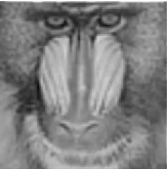
clear that the resulting image removes the blocking effect and staircase effects completely but as shown in Figure 4, this method has unpleasant blurring effects on the image.

(5)

(b) HR image with PDE

Figure 4. Blurring effects in HR image obtained from PDE.

Figure 5. Image enhancement by our proposed method without the problem of blurring effects as exists in Figure 4(b).

TABLE 1. Discretization used in the implementations.

±₍

, ) ±_∆ u ± i, j −u ,

±₍ _,₎ _±

∆ u ,± l −u ,

( , ) _∆ D (u ,)−D (u , )

±₍ _,₎ _±

∆ D ±(u ,±)−D ±(u , )

±₍

, ) ±_∆ D ±(u ±,)−D ±(u , )

( , ) _∆ D (u ,)−D (u , )

| ( , )| D u, + D u, + D u, + D u, +∈

In order to improve the proposed method and reduce the blur in the resulting image, the following points should be considered.

First, we apply a weighted averaging filter on image taken (LR image) before the computation of image zooming by LAZ algorithm. This filter is applied to the image once or twice. This is regarded a pre-processing operation.

u(i, j) = 2∗u(i, j) + u(i + 1, j) + u(i_{+u(i, j}₋_{1) + u(i, j + 1)}−1, j) 6 (15)

In addition, unsharp masking operation is applied to the HR image obtained from zooming by LAZ algorithm. Figure 5 shows this result. As you can see, blurred effect throughout the image has reduced dramatically and the result is an image with sharp edges.

It should be noted that the choice of an appropriate value for the parameters (ε, △x, △y) and time step (△t) is very important for the proposed method because if the value (△t) in an image is larger than the desired value, the image will not result in stable states through multiple repetitions. Furthermore, if the values of the parameters (ε, _△x, _△y) in an image are not properly determined, the image will be blocky. For this purpose, several trial and error experiments have been done to obtain the proper values on different images. The best value is designated for them as follows:△t = 10-3_,_△_{x =} △y = 0.7 and λ= 0, ε=10-4

4. PERFORMANCE METRICS

There are two types of the image quality assessment techniques. The objective methods result from the human judgment for evaluation of the image quality and subjective methods calculate the image qualities numerically. In this paper, both subjective and objective criteria are regarded in order to evaluate the performance of the proposed method. Four common objective methods used in this paper, are briefly introduced below.

4. 1. Figure of Merit Thefigure of Merit(FOM) criterion is used for the measurement of the preserved edges in the images and it is defined as follows [19]:

FOM = _{_, _}∑ _λ

(16)

Nz represents the number of edge pixels in zoomed image and No is the number of edge pixels of the original image. d iis the Euclidean distance between the i th_{edge pixel found and the nearest original edge pixel;}

(6)

4. 2. Structural SIMilarity Metric

The structural similarity metric (SSIM) proposed in [20] is based on human visual system. It consists of three different metrics. Let x, y be the original and the test images, respectively. SSIM is defined as:

SSIM = l(x, y)∗c(x, y)∗ ( , )

(17)

l(x, y)_μ μμ

μ

c(x, y) =

s(x, y) =

L measures how much the x and y are close in luminance. C measures the similarities between the contrasts of the images. S is the correlation coefficient between x and y, which measures the degree of linear correlation between them.

where,

μ = ∑ x , μ = ∑ y

(18)

σ = ∑(x − μ ) , σ =

∑ (y −μ )

σ = ∑ (x − μ )(y − μ )

The dynamic range of SIMM is [0, 1]. The best value, 1, is achieved if x=y.

Mean SSIM as the evaluation criteria is introduced. This metric can be implemented for an image as below:

MSSIM(x, y) =∑ SSIM(xj, yj) (19)

where, X and Y are the reference and the distorted images, respectively, M is the number of local windows in the image, SSIM is the Structural Similarity Index Matrix, xj and yj are the image contents at the jth local

window.

4. 3. Mean Square Error

Mean Square Error (MSE) metric is one of the simplest and oldest metric criteria that are defined asfollows:

MSE = ( _×)∑ ∑(M −N ) (20)

where, M and N denote the original image and zoomed image, respectively. K × L denotes both original and zoomed size images. In this metric, the smaller the MSE value, the better is the zoomed image performance.

4. 4. Peak-signal-to-noise The Peak-signal-to-noise (PSNR) is a well-known metric and is associated with MSE, it is defined as follows:

PSNR = 10log ^ dB (21)

Here, when the zoomed image has a higher PSNR value, it will be closer to the original image and will have a better quality.

5. NUMERICAL EXPERIMENTS

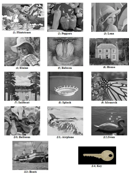
In this paper, we consider subjective and objective image quality assessment to evaluate the performance of the proposed algorithm. We also compare the results of our proposed method with four zooming methods described including LAZ [8], AZ [9], CIM [15] and BILI [5]. Firstly, the images shown in Figure 6 in [21] are zoomed out by 2 and 4 magnification factors and take them as LR image. Then, by applying the proposed method and four described algorithms to these LR images, they are multiplied by magnification factor of 2 and 4 and subsequently, they are compared with the original image again.

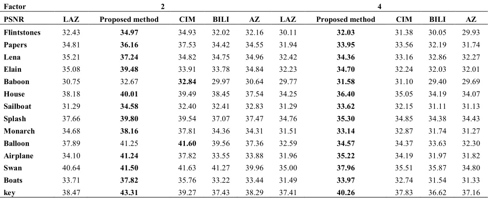
Table 2 and Table 4 show the values of criteria PSNR and FOM on 14 test images according to magnification factors. The proposed method has the maximum value of FOM and PSNR. As Table 3 show the values of criteria MSSIM on these images by magnification factor of 4. The MSSIM provides maximum value to the proposed algorithm.

(7)

TABLE 2. Values of measuring performance; FOM on 14 different image by magnification factor 2 and 4.

Factor 2 4

FOM LAZ Proposed method CIM BILI AZ LAZ Proposed method CIM BILI AZ

Flintstones 0.8873 0.9360 0.8464 0.8799 0.8486 0.5411 0.5997 0.5302 0.5377 0.4853

Papers 0.8652 0.8923 0.8503 0.8557 0.8415 0.5733 0.6705 0.6191 0.5829 0.5122

Lena 0.8686 0.9452 0.8102 0.8437 0.8405 0.5447 0.5988 0.5816 0.5603 0.4938

Elain 0.8678 0.9191 0.8370 0.8464 0.8431 0.544 0.6361 0.6048 0.5523 0.492

Baboon 0.8185 0.8321 0.7086 0.7754 0.7796 0.4121 0.5007 0.3852 0.3952 0.3562

House 0.9058 0.9077 0.8759 0.8994 0.8843 0.582 0.7502 0.6093 0.5697 0.5274

Sailboat 0.5044 0.9277 0.8708 0.8216 0.8169 0.5046 0.7148 0.5027 0.507 0.457

Splash 0.9132 0.9247 0.9229 0.9206 0.8999 0.6747 0.745 0.7298 0.7167 0.6673

Monarch 0.9012 0.9469 0.8843 0.8723 0.8768 0.6586 0.7306 0.7084 0.659 0.6181

Balloon 0.8734 0.9042 0.8863 0.8680 0.8486 0.5661 0.6388 0.6394 0.584 0.5001

Airplane 0.8840 0.8975 0.8452 0.8670 0.8631 0.5804 0.6766 0.5907 0.5751 0.5336

Swan 0.8300 0.8359 0.8048 0.8132 0.8049 0.4819 0.5458 0.4624 0.4903 0.4215

Boats 0.8296 0.8700 0.7919 0.8164 0.8049 0.5002 0.5796 0.4832 0.4822 0.4421

key 0.8213 0.9565 0.7393 0.7837 07880 0.5859 0.7543 0.522 0.5605 0.5322

TABLE 3.Values of measuring performance; MSSIM on 11 different images by magnification

Factor 4

MSSIM LAZ Proposed method CIM BILI AZ

Papers 0.8249 0.8634 0.8318 0.8200 0.8120

Lena 0.8015 0.8679 0.8166 0.8101 0.7881

Elain 0.8284 0.8752 0.8373 0.8176 0.8128

Baboon 0.5039 0.8596 0.7262 0.4587 0.5227

House 0.8234 0.8225 0.8486 0.8421 0.8091

Sailboat 0.7389 0.8673 0.7262 0.7288 0.7217

Splash 0.8616 0.8768 0.8628 0.8585 0.8542

Monarch 0.8584 0.8768 0.8565 0.8624 0.8458

Airplane 0.7716 0.8358 0.7555 0.7540 0.7563

Swan 0.8628 0.8971 0.8763 0.8763 0.8616

Boats 0.7247 0.8242 0.8031 0.7194 0.7061

TABLE 4. Values of measuring performance; PSNR on 14 different image by magnification factor 2 and 4.

Factor 2 4

PSNR LAZ Proposed method CIM BILI AZ LAZ Proposed method CIM BILI AZ

Flintstones 32.43 34.97 34.93 32.02 32.16 30.11 32.03 31.38 30.05 29.93

Papers 34.81 36.16 37.53 34.42 34.55 31.94 33.95 33.56 32.19 31.74

Lena 35.21 37.24 34.82 34.75 34.96 32.42 34.36 33.16 32.86 32.27

Elain 35.08 39.48 33.91 33.78 34.84 32.23 34.70 32.24 32.03 32.01

Baboon 30.75 32.67 32.84 29.97 30.64 29.77 31.58 31.10 29.40 29.69

House 38.18 40.01 39.49 38.45 37.54 34.25 36.40 35.05 34.19 34.07

Sailboat 31.29 34.58 32.40 32.41 32.83 31.29 33.62 32.15 31.11 31.13

Splash 37.66 39.80 39.54 37.07 37.47 34.76 35.30 34.85 34.38 34.43

Monarch 34.68 38.16 37.81 34.36 34.31 31.51 33.14 32.87 31.74 31.27

Balloon 37.89 41.25 41.60 39.56 37.36 32.59 34.57 34.37 33.63 32.30

Airplane 34.10 41.24 37.82 33.55 33.88 31.96 35.22 34.19 31.97 31.82

Swan 40.64 41.50 41.63 41.27 39.96 35.00 37.96 35.51 35.87 34.80

Boats 33.71 37.82 35.76 33.22 33.44 31.49 33.97 32.74 31.54 31.33

(8)

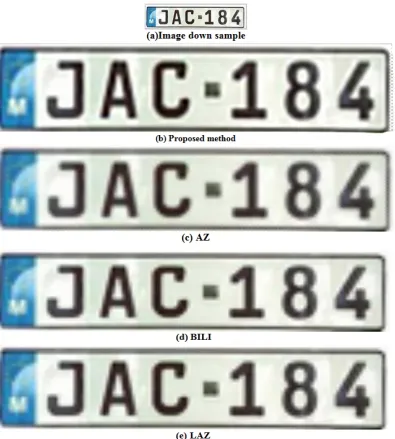
Figure 7.Results of the images zooming by factor 8 using (b) Proposed method, (c) AZ, (d) BILI, (e) LAZ.

The objective evaluation results indicate a better performance of the proposed method in maintaining edges and the quality of zoomed image than the four methods mentioned above. In addition, in Figure 7 the images of license plate have been zoomed by factor of 8. These results indicate the superiority of the proposed method over other methods.

As shown in Figure 8, images obtained by three methods (AZ, LAZ, and BILI), artifacts, blurring, blocking and staircase effects can be seen along the image edges while in the proposed method, they are reduced significantly. In addition, the proposed method had the best performance in the preservation of edges

and provides a sharp image that shows its superiority over CIM method.

(9)

(a) Original image (b) Proposed method

(c) CIM (d) LAZ

(e) BILI (f) AZ

(10)

(a) Proposed method, (FOM 0.6705 ¼ dB)

(b) CIM, (FOM 0.6191 ¼ dB)

(c) LAZ, (FOM 0.5733 ¼ dB)

(d) BILI, (FOM 0.5829 ¼ dB)

(e) AZ, (FOM 0.5122 ¼ dB)

Figure 9. Difference images of Elaine images shown in Figure (8).

(11)

(b) Proposed method,(PSNR 29.80¼ dB)

(c) LAZ ,(PSNR 29.57¼ dB)

(d) BILI,(PSNR 29.38¼ dB)

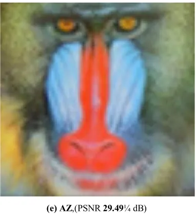
(e) AZ,(PSNR 29.49¼ dB)

Figure 10. (a) Original image and Results of the color images zooming by factor 4 using (b) Proposed method, (c) CIM, (d) LAZ, (e) BILI, (f) AZ.

(a) Original image

(12)

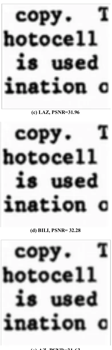
(c) LAZ, PSNR=31.96

(d) BILI, PSNR= 32.28

(e) AZ, PSNR=31.63

Figure 11. (a) Original image and Results of the textimages zooming by factor 4 using (b) Proposed method, (c) CIM, (d) LAZ, (e) BILI, (f) AZ.

The distortions are the white region of the difference images. The concentration of the distortion depends on the brightness of the area. In Figure 9, the white region is comparatively less obvious in the difference image of the proposed method (see in Figure 9 (a)). From visual observation of the zoomed images and FOM values in Figure 9, it can be concluded that the resulting image of the proposed method has well preserved the edges. Therefore, using difference image (objective assessment) shows that the proposed method is better in Figure 8.

To compare the proposed method with the present methods (LAZ, AZ, BILI), Figure 10 represents a sample of the color images with their PSNR values. High quality of the proposed method is visible with a subjective assessment of human observation and objective assessment with high values of PSNR. These images show that the PSNR values are in agreement with subjective evaluations of human observers. Among other examples in this paper to illustrate the effectiveness of the proposed method, zooming of Text image with factor 4 is in Figure 11. The result of zooming through the proposed method in Figure 11(b) shows a clearer Text image and is better than the other method in Figure 11 (c)-(e).

6. CONCLUSIONS

In this paper, a zooming method has been presented based on PDE. The proposed method is a combination of fourth-order PDE method with LAZ algorithm. During the process, known criteria of subjective and objective assessment were used. Results indicate that the proposed method is able to preserve the sharpness of the edges satisfactorily and minimize the artifacts such as image blur and staircase effects over the edge compared with LAZ method as well as other zooming methods explained in the article.

7. REFERENCES

1. Zhu, X., Lei, W. and Zhang, S., "Image zooming using c&e model and its performance evaluation", in Intelligent Control and Information Processing (ICICIP), International Conference on, IEEE. (2010), 262-265.

2. Combs, T. T. and Bederson, B. B., "Does zooming improve image browsing?", in Proceedings of the fourth ACM conference on Digital libraries, ACM. (1999), 130-137.

3. Almira, J. and Romero, A., "Image zooming based on sampling

theorems", MATerials MATematic, Vol. 2011, No. 1, (2011). 4. Lukac, R. and Plataniotis, K. N., "Bayer pattern based digital

zooming approach", in Circuits and Systems, ISCAS'04. Proceedings of the 2004 International Symposium on, IEEE. Vol. 3, No., (2004), III-253-6 Vol. 3.

5. Singh, C., Interpolation methods image zooming, in the National

(13)

6. Chadda, S., Kaur, N. and R., T., "Zooming techniques for digital images: A survey", InternatIonal Journal of Computer Science and Technology, Vol. 3, No. 1, (2012), 519-523.

7. Lehmann, T. M., Gonner, C. and Spitzer, K., "Survey:

Interpolation methods in medical image processing", Medical Imaging, IEEE Transactions on, Vol. 18, No. 11, (1999), 1049-1075.

8. Battiato, S., Gallo, G. and Stanco, F., "A locally adaptive zooming algorithm for digital images", Image and Vision Computing, Vol. 20, No. 11, (2002), 805-812.

9. Kumar, M., An adaptive zooming algorithm for images, in

computer science and engineering department. (2009).

10. Allebach, J. and Wong, P. W., "Edge-directed interpolation", in Image Processing, 1996. Proceedings., International Conference on, IEEE. Vol. 3, (1996), 707-710.

11. Li, X. and Orchard, M. T., "New edge-directed interpolation", Image Processing, IEEE Transactions on, Vol. 10, No. 10, (2001), 1521-1527.

12. Tam, W.-S., Kok, C.-W. and Siu, W.-C., "Modified edge-directed interpolation for images", Journal of Electronic Imaging, Vol. 19, No. 1, (2010), 013011-013011-20.

13. Wittman, T. C., Varational approaches to digital zooming, in University of Minnesota. (2006).

14. Guichard, F. and Malgouyres, F., "Total variation based interpolation", in Proceedings of the European signal processing conference, Citeseer. Vol. 3, No., (1998), 1741-1744.

15. Kim, H., Cha, Y. and Kim, S., "Curvature interpolation method for image zooming", Image Processing, IEEE Transactions on, Vol. 20, No. 7, (2011), 1895-1903.

16. Gao, R., Song, J.-P. and Tai, X.-C., "Image zooming algorithm based on partial differential equations technique", International Journal of Numerical Analysis and Modeling, Vol. 6, No. 2, (2009), 284-292.

17. Lysaker, M., Lundervold, A. and Tai, X.-C., "Noise removal using fourth-order partial differential equation with applications to medical magnetic resonance images in space and time", Image Processing, IEEE Transactions on, Vol. 12, No. 12, (2003), 1579-1590.

18. Lysaker, M. and Tai, X.-C., "Iterative image restoration combining total variation minimization and a second-order functional", International Journal of Computer Vision, Vol. 66, No. 1, (2006), 5-18.

19. Jähne, B., "Digital image processing", Measurement Science and Technology, Vol. 13, No. 9, (2002), 1503.

20. Wang, Z., Bovik, A. C., Sheikh, H. R. and Simoncelli, E. P., "Image quality assessment: From error visibility to structural similarity", Image Processing, IEEE Transactions on, Vol. 13, No. 4, (2004), 600-612.

21. Available from: www.freeimages.co.uk and

(14)