SHEAR-WAVE DYNAMIC BEHAVIOR USING
TWO DIFFERENT ORIENTATIONS
Mohammad Kamal Ghassem Alaskari
Department of Petroleum Engineering, Petroleum University of Technology P. O. Box 63431, Ahwaz, Iran
Seyed Jalaladdin Hashemi*
Department of petroleum Engineering, PUT and Islamic Azad University-Ahvaz Branch Ahvaz, Iran
[email protected] – [email protected]
*Corresponding Author
(Received: October 12, 2006 – Accepted in Revised Form: September 13, 2007)
Abstract For laterally complex media, it may be more suitable to take a different orientation of the displacement vector of Shear-waves. This may change the sign of several imaginary reflections and conversion coefficients to be used in reservoir characterization and AVO (Amplitude Versus Offset) analysis or modeling. In this new convention the positive direction of the displacement vector of reflected Shear-waves is chosen to the left of ray tangent (in the direction of wave propagation). Therefore, the definition of the displacement vector of shear-waves can be used properly even for very complicated media. Finally the shear-wave dynamic behavior of a reservoir zone can be illustrated for laterally varying structures in terms of the amplitude variation and phase behavior using this new orientation.
Keywords Shear-Wave, Dynamic Behavior, Two Different Orientations
ﻩﺪﻴﻜﭼ
ﺖﺳﺍﺮﺘﻬﺑ،ﯽﺒﻧﺎﺟﺕﺍﺮﻴﻴﻐﺗﯼﺍﺭﺍﺩﻩﺪﻴﭽﻴﭘﯽﻧﺎﻤﺘﺧﺎﺳﯼﺎﻫﻂﻴﺤﻣﺭﺩﺭﻮـﻈﻨﻣﻪﺑ
ﺕﺍﺭﺫﯽﺋﺎـﺠﺑﺎﺟ ،
ﻂﻴـﺤﻣ
ﺩﻮﺷﺏﺎﺨﺘﻧﺍﻝﻭﺍﺪﺘﻣﺖﻬﺟﺯﺍﺮﻴﻏﯽﺘﻬﺟﺭﺩﯽﺷﺮﺑﺝﺍﻮﻣﺍﻂﺳﻮﺗ .
ﯽﻣﻮـﻫﻮﻣﺖﻳﺍﺮـﺿﺖـﻣﻼﻋ،ﺖـﻬﺟﺮـﻴﻴﻐﺗﻦﻳﺍ
ﯽﻣﺮﻴﻴﻐﺗﺍﺭﯽﻠﻳﺪﺒﺗﻭﯽﺑﺎﺗﺯﺎﺑﺝﺍﻮﻣﺍ
ﻴﻠﺤﺗﻭﻥﺰﺨﻣﺕﺎﻴﺻﻮﺼﺧﻦﻴﻴﻐﺗﺭﺩﻪﮐﺪﻫﺩ ﯼﺎـﻫﻝﺪﻣﻞ
AVO ﺮﺛﻮـﻣﺭﺎﻴﺴـﺑ
ﺖﺳﺍ . ﺝﻮـﻣﺭﺎﺸـﺘﻧﺍﻪﺤﻔﺻﺭﺩﻪﮐﻩﺪﺷﺏﺎﺨﺘﻧﺍﯼﺍﻪﻧﻮﮕﺑﻦﻳﻭﺪﺗﻦﻳﺍﺭﺩﯽﺷﺮﺑﺝﺍﻮﻣﺍﯽﺋﺎﺠﺑﺎﺟﺭﺍﺩﺮﺑﺖﺒﺜﻣﺖﻬﺟ
ﺩﻮﺷﻊﻗﺍﻭﻮﺗﺮﭘﭗﭼﺖﻤﺳﺭﺩ .
ﺐـﺟﻮﻣﯽﺒﻧﺎﺟﯽﻧﺎﻤﺘﺧﺎﺳﺕﺍﺮﻴﻴﻐﺗﺎﺑﯽﻧﺰﺨﻣﻪﻴﺣﺎﻧﺭﺩﯽﺷﺮﺑﺝﻮﻣﯽﮑﻴﻣﺎﻨﻳﺩﺭﺎﺘﻓﺭ
ﯽﻣﺝﻮﻣﺯﺎﻓﻭﻪﻨﻣﺍﺩﺕﺍﺮﻴﻴﻐﺗ
ﻦﻳﻭﺪﺗﺎﺑﻪﮐﺩﻮﺷ
ﺩﺭﺍﺩﺖﻘﺑﺎﻄﻣﺮﺘﻬﺑﺪﻳﺪﺟ .
ﯼﺎـﻫﻂﻴـﺤﻣﯼﺍﺮـﺑﻦﻳﻭﺪﺗﻦﻳﺍﻭﺭﻦﻳﺍﺯﺍ
ﺖﺳﺍﺮﺗﺐﺳﺎﻨﺘﻣﻩﺪﻴﭽﻴﭘﯽﻧﺎﻤﺘﺧﺎﺳ .
1. INTRODUCTION
The crucial importance of shear waves as well as P to S conversion waves and their applications in seismology led to the investigation of the dynamic properties (i.e. reflection, transmission, conversion coefficients, amplitude ratios and phase behavior) in terms of angles of incidence.
Since 1919 the complex plane wave reflection and transmission coefficients given by Zoeppritz were sometimes erroneously used due to different notations and sign orientations. Some of these
errors are reported by Hales and Roberts [1], other errors have been found in reference [2].
The sixteen explicit plane wave reflection and transmission coefficients of P and SV-waves between two homogeneous media are given by Cerveny and Ravindra [3]. These coefficients are rewritten by Cerveny et al. [4] with a different notation for plane boundaries and applied by Rectora, et al. [6], and Marra, et al. [7].
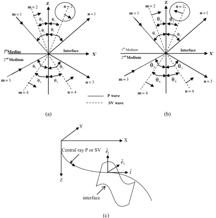
such a way that its projection on the x-axis is positive (Figure 1a). Its implication is that the displacement vector of SV-wave may change sign at certain points of the ray and (-1) multiplier must be introduced. In this research paper the Fuchs’ convention [5], Cerveny’s convention [3,4] and modified versions [2] are compared computationally.
2. GOVERNING EQUATIONS
In order to determine the general solutions of P-SV reflection and transmission coefficients suitable for inhomogeneous media with planar boundaries, the sixteen explicit coefficients (Figure 1a) given by Cerveny (1971) can be written as follows.
For downgoing P-waves;
D / Z 2 1 3 P 2 P q 1 P P 1 1 2 14 R D / Y 4 P 1 X 2 P 2 1 P 1 1 2 13 R D / XZ 2 2 Y 4 P 3 P q 1 PP 1 2 12 R D / 4 P 3 P 2 P 2 P 2 q 4 P 2 1 2 1 2 X 2 P 2 2 1 P 2 1 11 R ⎟ ⎠ ⎞ ⎜ ⎝
⎛ −β α
ρ α − = ⎟ ⎠ ⎞ ⎜ ⎝
⎛β +β
ρ α = ⎟ ⎠ ⎞ ⎜ ⎝
⎛ +α β
α − = ⎟ ⎠ ⎞ ⎜ ⎝
⎛α β +β α ρ ρ +
+ − =
(1a) For downgoing SV-waves;
D / X 1 P 2 Y 3 P 1 2 P 1 1 2 24 R D / Z 1 2 4 P 1 P q 2 PP 1 1 2 23 R D / 4 P 3 P 1 P 2 P 2 q 3 P 2 1 1 2 2 X 1 P 2 2 2 P 2 1 22 R D / XZ 2 2 Y 4 P 3 P q 2 PP 1 2 21 R ⎟ ⎠ ⎞ ⎜ ⎝
⎛α +α
ρ β = ⎟ ⎠ ⎞ ⎜ ⎝
⎛ −β α
ρ β = ⎟ ⎠ ⎞ ⎜ ⎝
⎛α β +β α ρ ρ +
− = ⎟ ⎠ ⎞ ⎜ ⎝
⎛ +β α
β − =
(1b)
For upgoing P-waves;
D / Z 2 2 4 P 1 P q P 3 P 2 2 2 32 R D / Y 4 P 1 X 2 P 2 3 P 2 2 2 31 R ⎟ ⎠ ⎞ ⎜ ⎝
⎛ −α β
ρ α = ⎟ ⎠ ⎞ ⎜ ⎝
⎛β +β
ρ α = D / YZ 1 1 X 2 P 1 P q 3 PP 2 2 34 R D / 4 P 2 P 1 P 2 P 2 q 2 P 2 1 2 1 2 Y 4 P 1 1 3 P 2 1 33 R ⎟ ⎠ ⎞ ⎜ ⎝
⎛ +αβ
α = ⎟ ⎠ ⎞ ⎜ ⎝
⎛α β +α β ρρ + +
− =
(1c)
And for upgoing SV-waves;
D / 3 P 2 P 1 P 2 q 1 P 2 1 1 2 2 Y 3 P 1 1 4 P 2 1 44 R D / YZ 1 1 X 2 P 1 P q 4 PP 2 2 43 R D / Y 3 P 1 X 1 P 2 4 P 2 2 2 42 R D / Z 1 2 3 P 2 P q 4 PP 2 2 2 41 R ⎟ ⎠ ⎞ ⎜ ⎝
⎛α β +α β ρρ +
− = ⎟ ⎠ ⎞ ⎜ ⎝
⎛ +αβ
β = ⎟ ⎠ ⎞ ⎜ ⎝
⎛α +α
ρ β = ⎟ ⎠ ⎞ ⎜ ⎝
⎛ −α β
ρ β = (1d) Where, 4 Cos 2 1 ) 2 P 2 2 1 ( 4 P , 3 Cos 2 1 ) 2 P 2 2 1 ( 3 P , 2 Cos 2 1 ) 2 P 2 1 1 ( 2 P , 1 Cos 2 1 ) 2 P 2 1 1 ( 1 P ), 2 P q 1 2 ( Z ), 2 qP 1 ( Y ), 2 P q 2 ( X , j V / j Sin P ), 2 1 1 2 2 2 ( 2 q 2 X 2 2 4 P 3 P 2 P 2 q ( 2 P 1 P ) 2 Z 2 P 2 2 2 Y 4 P 3 P ( 1 1 3 P 2 P 2 1 4 P 1 P 2 1 2 1 D θ = β − = θ = α − = θ = β − = θ = α − = − ρ − ρ = + ρ = − ρ = θ = β ρ − β ρ = ⎟ ⎠ ⎞ β α + + β α ⎜ ⎝
⎛β α +α β +α β +
ρ ρ =
Equations 1 can be modified for the new sign convention according to Figure 1b as the followong eight explicit forms;
For downgoing P-waves;
D / Z 2 1 3 P 2 P q 1 P P 1 1 2 14 R D / Y 4 P 1 X 2 P 2 1 P 1 1 2 13 R D / XZ 2 2 Y 4 P 3 P q 1 PP 1 2 12 R D / )] 2 X 2 2 4 P 3 P 2 P 2 q ( 2 P 1 P ) 2 Z 2 P 2 2 2 Y 4 P 3 P ( 1 1 ) 3 P 2 P 1 2 4 P 1 P 1 2 ( 2 1 [ 11 R ⎟ ⎠ ⎞ ⎜ ⎝
⎛ −βα
ρ α − = ⎟ ⎠ ⎞ ⎜ ⎝
⎛β +β ρ α = ⎟ ⎠ ⎞ ⎜ ⎝
⎛ +αβ
For downgoing SV-waves; D / X 1 P 2 Y 3 P 1 2 P 1 1 2 24 R D / 4 P 1 P q Z 1 2 2 PP 1 1 2 23 R D / )] 2 X 2 2 4 P 3 P 2 P 2 q ( 2 P 1 P ) 2 Z 2 P 2 2 2 Y 4 P 3 P ( 1 1 ) 4 P 1 P 2 1 3 P 2 P 2 1 ( 2 1 [ 22 R D / XZ 2 2 Y 4 P 3 P q 2 PP 1 2 21 R ⎟ ⎠ ⎞ ⎜ ⎝
⎛α +α ρ β = ⎟ ⎠ ⎞ ⎜ ⎝
⎛β α − ρ β − = β α + + β α + β α − α β − β α ρ ρ = ⎟ ⎠ ⎞ ⎜ ⎝
⎛ +β α
β − =
(2b)
Therefore, for a laterally inhomogeneous medium with planar boundaries (Figure 1c), the Equations 2 can be used instead of corresponding R-coefficients in the Equations 1.
For P>1 αj, all Pj in Equations 1 and 2 must
be replaced by 2 1)12 j V 2 P ( i j
P =m − , respectively for j = 1 to 4, i.e. minus sign must be used with Equations 1 and plus sign with Equations 2.
Where; V1=α1, V2 =β1, V3=α2, V4=β2 and
1
i= − are used for each interface between two media (V1=α1, V3=α2 are P-wave and V2=β1,
2 4
V =β are S-wave velocities) and ρ is the density. Note that the sign convention for Cerveny’s notations and Alaskari’s notations are chosen according to Figures 1a and 1b, respectively.
If the receiver is located on the surface of the earth, it is necessary to consider both the incident and the interference waves (generated at the free surface) and the reflection coeffcients:
B / ] 2 P 2 1 2 1 1 / 2 1 2 P P 4 [ 21 R B / ] 2 2 P 2 1 2 1 1 / 3 1 2 P 1 P 2 4 [ 22 R B / 2 P 2 1 2 1 1 PP 1 4 12 R B / ] 1 / 3 1 2 P 1 P 2 P 4 2 ) 2 P 2 1 2 1 ( [ 11 R ⎟ ⎠ ⎞ ⎜ ⎝ ⎛ − β α β = ⎟ ⎠ ⎞ ⎜ ⎝ ⎛ − β − α β ρ = ⎟ ⎠ ⎞ ⎜ ⎝ ⎛ − β β − = α β + β − − =
A common situation in exploration seismology is that the receiver is located on the surface of the earth. Therefore the Hilbert transformation of the
source function must be slightly modified according to new convention. Beside for the incident P to S waves, the generated waves at the free surface must also be considered, which interference occurs. To obtain the interferences, it will be better to introduce the so called conversion vector qr as follow (Figure 1c);
For incident P-wave;
2 eˆ 12 R 1 eˆ 11 R tˆ
qr= + +
For incident SV-wave;
2 eˆ 22 R 1 eˆ 21 R tˆ
qr= + +
The system of local ray coordinates is chosen as shown in Figure 1c. For the implication of the above conversion vector in the source term see refrence [8]. The components of the conversion vector corresponding to the local coordinate system are called the conversion coefficients (i.e.
z q , y
q ) and can be written as follows; For incident P-wave;
B ) 2 P 2 1 2 1 ( 1 P 2 Z q B P 2 P 1 P 1 4 y
q = β =− − β (3)
For incident SV-wave;
B 1 P 2 P 1 P 2 1 4 Z q B ) 2 P 2 1 2 1 ( 2 P 2 y
q = − β = β α (4)
where B is called Rayleigh function and is given by; 1 ) 2 P 1 P 2 P 3 1 4 ( ) 2 P 2 1 2 1 (
B= − β + β α (5)
wave SV
wave P
1
θ
1
θ
1
=
m n=1
3
=
m n=3
3 θ 3
θ
4
=
m n=4
4 θ θ4
Z
` X Interface Medium
1St
Medium
nd
2
2 θ θ2
2
=
m n=2
1
=
m n=1
3
θ
4
θ
1
θ
1
θ
2
θ θ2
4
θ
3
=
m n=3
4
=
m n=4
3
θ
2
=
m Z n=2
` X Interface
Medium St 1
Medium
nd
2
(a) (b)
1 ˆ e 2 ˆ e
tˆ
X Y
Z
interface Central ray P or SV
(c)
Figure 1. Sign convention of Reflection and Transmission Coefficients for incident P and S-waves, the changes are high-lighted by circles. (a) Standard sign convention, (b) Modified sign convention
(c) 3D-ray representation of central-ray at the curved interface.
matching method. θj=Sin−1(V0Pj), where j = 3 for P-waves and j = 4 for SV-waves, i.e.
) 4 , 3 P 0 V ( 1 Sin 4 ,
3 = −
θ .
Note that in the definition of Equations 1 the positive direction of the displacement vector of the SV-wave is chosen such that its projection on the
shear-TABLE 1. Test Models.
Mathematical Models (Single Layer Over a Half Space) (1) Low Velocity Contrast
(M1-Cerveny, 1971)
(2) High Velocity Contrast (M2-Cerveny, 1971)
(3) Average Crust Model (M3-Alaskari, 1983)
HZ 10 0 f
km 30 crust Average
3 cm / g 3 . 3 2
3 cm / g 0 . 3 1
732 . 1 VS VP
sec / km 0 . 8 2 VP
sec / km 4 . 6 1 VP
=
= =
ρ = ρ
= = =
Zero-phase
HZ 50 0 f
km 0 . 1 reflector of
Depth
3 cm / g 0 . 4 2
3 cm / g 0 . 3 1
732 . 1 VS VP
sec / km 0 . 5 2 VP
sec / km 0 . 2 1 VP
=
= =
ρ = ρ
= = =
Zero-phase
HZ 10 0 f
km 30 crust Average
3 cm / g 3 . 3 2
3 cm / g 0 . 3 1
732 . 1 VS VP
sec / km 2 . 8 2 VP
sec / km 5 . 6 1 VP
=
= =
ρ = ρ
= = =
Zero-phase wave reflection coefficients (Figure 1b). For
example, in definition of the modified Equations 2 the particle motion was chosen on the displacement vector of the SV-wave to the left of the tangent to the ray (in direction of propagation) as positive. This convention is more suitable for applying the R-coefficients in laterally as well as vertically varying media [2].
This is properly defined and remains well defined even for very complicated rays in laterally varying media. The modulus of the R-coefficients in both cases are of course, the same (see Figure 2b), but the shear-wave reflection coefficients have different signs convention. Note that according to governing Equations 2, the above mentioned R-coefficients must be used very carefully(Figure 1c).
3. SYNOPSIS
To check the signs of the R-Coefficients and the sensitivity of the dynamic properties of seismic body waves, three different Algorithms were tested [2]. Three model examples (Table 1) are illustrated
in this paper to verify the conversion coefficients (Figures 2a and 3). In these examples the R-coefficient of P and SV incident waves on an elastic discontinuous medium were calculated on CDC 6600 (Mainframe) for all real angles of incidence, which varied from 0 to 90 degrees, in one degree increment except near the critical angle, where the coefficients were computed at 0.25 degree increments.
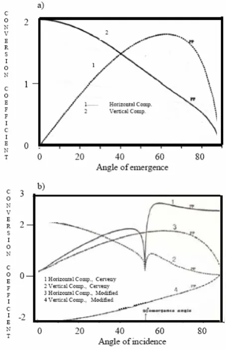
In this investigation both real and imaginary coefficients were considered in the computations. The modulus of the reflected P-wave for models 1 and 2 are compared in Figure 2b. In Figure 2a the surface conversion coefficients are computed for the models 1 and 2 (see Table 1).
These types of coefficients should be replaced by tangential vectors in order to correct the effect of wave interference for the receivers located on the earth’s surface. The curves in Figures 2a and 3a are plotted for the real angles of incidence whose reflection and transmission coefficients are real and that portion of plots whose reflection and transmission coefficients become imaginary are omitted.
Figure 2. Coefficients computed for the models 1 and 2 given in Table 1, (a) Surface conversion coefficients, (b) Modulus of the P-wave reflection.
Figure 3. The vertical and horizontal components of conversion coeficients computed for the model 3 given in Table 1. For angles of emergence only, For angles of incidence compared to angles of emergence.
horizontal and vertical components of the P-wave conversion coefficients are zero at critical angle for the Cerveny’s conventions and the horizontal and vertical components of the P-wave conversion coefficients are not zero for modified version. The computed conversion coefficients for the same model (model 3) shown in Figure 3b are plotted for the emergence angles. In Figure 3-a the arrow represents the 90 degree emergence angle for incoming waves corresponding to the critical angle. As seen in Figure 3a the P-wave conversion coefficients using the modified version is not
singular at the critical angle (52.4).
Figure 4. R-coefficients computed for the model 3 given in Table 1 (a) Fuchs’,(b) Cerveny’s, (c) Modified.
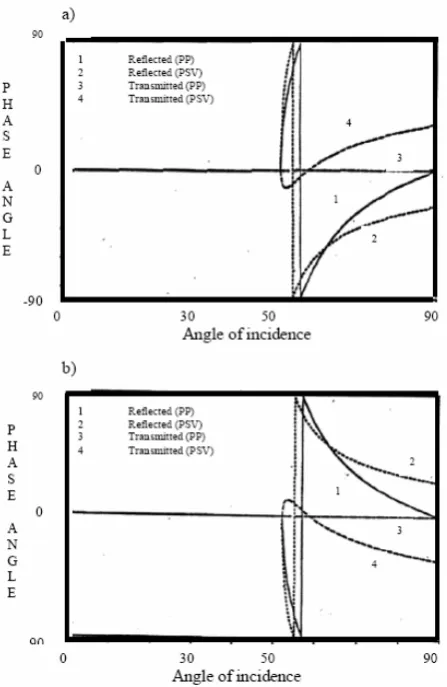
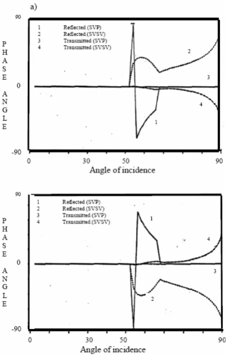
Figure 5. The phase angles of reflected and transmitted waves for model 3. (a) Cerveny’s formula, (b) The modified formula.
The phase angles of reflected and transmitted waves are computed for the model 3 using standard and modified fotmulae in Figures 5 and 6. As it can be seen from Figures 5 and 6 the phases for all generated waves at the subcritical angles are zero. The P to P, P to SV and SV to P, SV to SV reflected waves have rapid phase changes at the critical angles. The P to P and SV to P transmitted
waves have no phase changes for all angles of incidence, but the P to SV and SV to SV transmitted waves have phase changes in the post-critical angles.
In Figure 5b and 6b all coefficients have opposite signs for all angles of incidence compared to Figures 5a and 6a, except for the P to P and SV to P transmitted waves.
4. CONCLUSION
Figure 6. The reflected phase angle versus angle of incidence for model 3. (a) Cerveny’s formula, (b) The modified formula.
density ratio, but changes in the velocity ratio may cause significant changes in amplitude ratios. At the critical angle, the amplitude ratios of reflected waves change rapidly and approach its maximum. Beyond the critical angle small changes in velocity ratio (VP VS) may have effect on the amplitude ratio. Therefore, it is more suitable to apply the modified R-coefficients given in Equation 2 for reservoir characterization, AVO analysis and AVO modeling.
In conclusion for the two different orientations mentioned in this paper, the modulus of reflection
and transmission coefficients are, of course, the same. Beyond the first critical angles, the amplitudes of the generated waves are complex, and all waves undergo phase changes. The phase changes near the critical angles are often large and rapid.
The significance of a phase change in the generated wave is to change the arrival time of a peak or trough of the wave. The amount of delay or advance in reservoir characterization can be interpreted as negative or positive phase change respectively. This type of shear wave application would include the correction of observed travel times by the appropriate delay or advance time, determined from the phase angle in order to locate the depth of reflectors more precisely for laterally varying structures. The verification of the new sign convention against the field data will be illustrated in the future comming paper.
5. REFERENCES
1. Hales, A. and Roberts, L., “The Zoeppritz Amplitude Equation more Errors”, SSA, Vol. 64, (1974), 285.
2. Ghassem Alaskari, M. K., “The R-Coefficients for the two different orientations, in Department of Geological Sciences”, Southern Methodist University, Dallas, TX, 75275, USA, (1981).
3. Cerveny, V. and Ravindra, R., “Theory of seismic head waves”, Toronto: University of Toronto, Press, (1971). 4. Cerveny, V., Molotkov, I. and Psencik, I., “Ray Method
in Seismology”, ed. C. U. Press., Prague, (1977). 5. Fuchs, K., “The Rrflection of Spherical Waves from
Transmission Zone with Arbitrary Depth-Dependent Elastic Modulus and Density”, Journal of Physics of Earth, Vol. 16, (1968), 27-41.
6. Rechor, J. W., Lazaratos, S. K., Harris, J. M. and Van Schaack, M., “High resolution cross well imaging of a West Texas carbonate reservoir, Part-3 Reflection Wavefield Separation”, Geophysics, Vol. 60, (1995),
692-701.
7. Marra, A., Perez, V. G. and Reinaldo J., “Michelena, Fracture detection in a Carbonate resevoir using a variety of seismic methods”, Geophysics, Vol. 64, No.
4, (1999), 1266-1276.
8. Ghassem Alaskari, M. K. and Hashemi, S. J., “An Efficient Algorithm for General 3D-Seismic Body Waves (SSP and VSP Applications)”, International Journal of Engineering, Vol. 18, No. 4, (2005),