On imputation for planned missing data in context questionnaires using plausible values: a comparison of three designs

(1)

On imputation for planned missing data

in context questionnaires using plausible values:

a comparison of three designs

David Kaplan

*

_{and Dan Su}

Introduction

A recent paper by Kaplan and Su (2016) investigated the problem of matrix sampling of context questionnaires with respect to the generation of the plausible values (PVs) of the so-called “cognitive” tests in large-scale educational assessments. Drawing on earlier work by Adams et al. (2013) based on PISA 2012 OECD (2014) and motivated by the desire among policy-makers to increase non-cognitive content in national and international large-scale assessments, Kaplan and Su found that matrix sampling of con-text questionnaire (CQ) material followed by predictive mean matching imputation can

Abstract

Background: This paper extends a recent study by Kaplan and Su (J Educ Behav Stat 41: 51–80, 2016) examining the problem of matrix sampling of context questionnaire scales with respect to the generation of plausible values of cognitive outcomes in large-scale assessments.

Methods: Following Weirich et al. (Nested multiple imputation in large-scale assess-ments. In: Large-scale assessments in education, 2. http://www.large scale asses sment sined ucati on.com/conte nt/2/1/9, 2014) we examine single + multiple imputation and multiple + multiple imputation methods using predictive mean matching imputa-tion under three different context quesimputa-tionnaire matrix sampling designs: a two-form design studied by Adams et al. (On the use of rotated context questionnaires in conjunction with multilevel item response models. In: Large-scale assessments in education. http://www.large scale asses sment sined ucati on.com/conte nt/1/1/5, 2013), a three-form design implemented in PISA 2012, and a partially-balanced incomplete design studied by Kaplan and Su (J Educ Behav Stat 41: 51–80, 2016).

Results: Our results show that the choice of design has a larger impact on the reduc-tion of bias than the choice of imputareduc-tion method. Specifically, the three-form design used in PISA 2012 yields considerably less bias compared to the two-form design and the partially balanced incomplete design. We further show that the partially balanced incomplete block design produces less bias than the two-form design despite having the same amount of missing data.

Conclusions: We discuss the results in terms of implications for the design of context questionnaires in large-scale assessments.

Open Access

© The Author(s) 2018. This article is distributed under the terms of the Creative Commons Attribution 4.0 International License (http://creat iveco mmons .org/licen ses/by/4.0/), which permits unrestricted use, distribution, and reproduction in any medium, provided you give appropriate credit to the original author(s) and the source, provide a link to the Creative Commons license, and indicate if changes were made.

RESEARCH

(2)

quite accurately recover the known marginal distributions of the PVs. However, bias was found in the estimation of correlations between CQ scales and PVs.1_{Kaplan and} Su (2016) speculated that this bias was due to the fact that the plausible values were not part of the missing data imputation model and hence not “congenial” in the sense of Meng (1994).

In this paper, we investigate two approaches to multiple imputation that use PVs in the imputation model for the missing CQ data. To our knowledge, the two approaches discussed in Weirich et al. (2014) have not been studied across different missing data designs, and so an important feature of this paper is that we compare these approaches under three planned missing data designs: a two-form design examined by Adams et al. (2013), a three-form design that was used for PISA 2012, and a partially balanced incom-plete block design (PBIB) studied by Kaplan and Su (2016). We carry out our investiga-tion by simulating these designs on data from PISA 2006, allowing a comparison of our findings to the actual empirical data. We evaluate the marginal distributions of the PVs, the correlations among the imputed CQ variables and the PVs as well as the estimates of regression coefficients and their corresponding standard errors, by comparing to the original questionnaire without matrix sampling and imputation.

The organization of this paper is as follows. In the next section, we provide a review of the literature on missing data in large-scale assessments by first suggesting that prior research on the topic can be situated within the framework of congenial missing data problems. This is followed by an overview of the matrix sampling designs used in this study. This is then followed by a description of the simulation design for this paper. Next, we provide the results of our simulation studies focusing on recovery of marginal distri-butions of PVs, bias in the correlations among the CQ and PVs, and bias in regression coefficients and their standard errors from a regression of the PVs on the CQ scales. The paper closes with a discussion of the results in light of recent calls for increased focus on the policy importance of context questionnaires in large-scale assessments.

Background

As noted earlier, one finding of the Kaplan and Su (2016) paper was that correlations among the PVs and imputed CQ scales were biased. Kaplan and Su speculated that this bias was due, in part, to the fact that the PVs themselves were not included in the impu-tation models that they explored. Omitting the PVs as part of the impuimpu-tation process leads to uncongeniality between the imputation model and the analysis model. This is a particular problem for secondary analyses of large-scale assessments insofar as the PVs of the cognitive assessments are, arguably, of primary policy importance.

Congenial missing data problems

We situate our discussion of imputation under planned missing data within the frame-work of congenial missing data problems. The concept of congeniality in missing data problems was introduced by Meng (1994), (see also; Rubin (1996)). In outlining the steps in conducting a large-scale survey, Meng (1994) pointed out that each step in the

1 _{For this paper, we focus on scales rather than the items that make up the scales. Matrix sampling of items within}

(3)

construction of a large-scale survey inherits information from the previous step. That is, the data file that a researcher uses is the result of a set of design steps which includes, in important ways, decisions that are made regarding the imputation of missing data. In many cases, as Meng (1994) notes, the individual (or individuals) charged with decisions regarding missing data imputation has little or no contact with the end-user of the data. Thus, if an analyst is interested in conducting some secondary statistical analysis using the data, his/her statistical model may have little in common with the model used to impute the missing data and this “disconnect” can lead to serious biases. Quoting Meng (1994, p. 539)

“...uncongeniality... essentially means that the analysis procedure does not corre-spond to the imputation model. The uncongeniality arises when the analyst and the imputer have access to different amounts and sources of information, and have dif-ferent assessments (e.g., explicit model, implicit judgement) about both responses and non-responses. If the imputer’s assessment is far from reality, then, as Rubin (1995)2_{wrote, “all methods for handling nonresponse are in trouble” based on such} an assessment; all statistical inferences need underlying key assumptions to hold at least approximately. If the imputer’s model is reasonably accurate, then following the multiple-imputation recipe prevents the analyst from producing inferences with serious nonresponse biases.”

The problem of uncongeniality has led to the general principle that one should include as many variables as possible in the imputation model for the missing data (see e.g. Rubin (1996)). Considering that the PVs in the various knowledge domains are a central focus of large-scale assessments, one purpose of this paper is to examine how PVs can be generated and used in the imputation of planned missing CQ data under different imputation methods and different designs and how these methods and designs impact the potential biases in secondary analyses.

Related research

Much of the extant literature addressing the topic of missing data in the CQ has focused on its impact with respect to the model used in generating population and sub-popu-lation ability estimates of plausible values (e.g. Mislevy (1991); von Davier et al. (2009); Rutkowski (2011)) and on item or variable non-response (e.g. Aßman et al. (2015)). The general finding is that sub-population estimates of plausible values are relatively stable under conditions of missing-at-random and not-missing-at random (Rutkowski 2011). The present paper continues along the line of inquiry found in von Davier (2014) and Kaplan and Su (2016) focusing on planned missing data arising from a deliberate matrix sampling of the CQ. As noted earlier, we extend on this current work by examining alter-native planned missing data designs and by examining alteralter-native approaches to imput-ing missimput-ing data in the CQ.

There are many approaches to addressing missing data in the CQ when generating PVs. A rather ad hoc method implemented in PISA is to use country means for missing values and create dummy codes to indicate missingness in the CQ. This is then followed

(4)

by a principal components analysis to reduce dimensionality and ease the computation of the PVs. The difficulty with the dummy coding approach, as pointed out by Aßman et al. (2015), is that it does not incorporate the PVs as part of the CQ imputation. This, in turn, results in an uncongenial missing data model and also does not address uncer-tainty arising from the missing data in the CQ. To explicitly address unceruncer-tainty arising from the missing data requires the use of multiple imputation methods (Rubin 1987). In principle, non-parametric or parametric methods can be used, however the question remains how the PVs can be incorporated into the imputation of the CQ missing data.

Rather than using dummy variables that are coded to address missing data, a general approach to incorporating PVs into the imputation of the CQ is through the use of mul-tiple imputation (Rubin 1987). A discussion of multiple imputation using PVs for CQ imputation was provided by Weirich et al. (2014). In their paper, Weirich et al. (2014) distinguish between two approaches to multiple imputation in this context: single+ mul-tiple imputation (SMI) and multiple+ multiple imputation (MMI). Following Weirich et al. (2014), four steps are required for the SMI approach. The first step is to create a of the item response model for the cognitive assessment without the use of the CQ. A sim-ple marginal maximum likelihood approach can be used for this step. The second step involves imputation of the CQ using a proxy for the latent ability θ . Proxies could include simple percentage correct, maximum likelihood estimates (MLEs), or Warm weighted likelihood estimates (WLEs; Warm (1989)). However, should be noted that these prox-ies are biased estimates of latent ability. Indeed, an important contribution of our paper is that we will use the generated PVs directly in the imputation of the CQ. The third step requires estimating the parameters of a latent regression model in which the latent ability variable is regressed on the set of CQ variables, where the CQ is now completed due to the imputation from the second step. This step is required in order to impute plausible values of the latent ability distribution and is standard procedure in large-scale assessments (see, e.g. von Davier (2014)).3_{The fourth step is the generation of the PVs} based on a “completed” CQ.

As shown by Weirich et al. (2014), the SMI approach does reduce bias in the popula-tion model when the uncertainty in the CQ depends on θ . However, as they also note, the SMI approach is still not optimal because there exists uncertainty in the estimation of θ due to missingness in the CQ. To fully address this uncertainty, Weirich et al. (2014) advocate for the MMI approach. The MMI approach is based on the notion of nested (or two-stage) multiple imputation developed by Rubin (2003), (see also; Schafer and Graham (2002); Reiter and Raghunathan (2007); Harel (2007)). The basic steps of MMI require that in the second step described for SMI, M imputations of the CQ are created. Step 3, then, must be repeated M times, and then this is followed by Step 4 where, say, K plausible values are drawn from the posterior distribution of latent ability resulting in M×K plausible values. As noted by Rubin (2003, p. 6), the usual combining rules under multiple imputation must be modified because nested imputations are correlated.

In an extensive simulation study, Weirich et al. (2014) found that the SMI and MMI approaches provided roughly comparable reduction of bias in the population model.

(5)

They go on to suggest that one limitation of their study was the use of the WLEs as prox-ies for θ . As noted by Wu (2005), the problem with using WLEs as proxies for θ is that it is a biased estimate of the population mean unless the same test items are given to all respondents—which is not the case with international large-scale assessments such as PISA which utilize a balanced incomplete-block spiraling design for test booklets. More-over, as pointed out by Mislevy et al. (1992), WLEs are susceptible to scale unreliability. We address the problem of using WLEs by estimating PVs directly in the imputation process.

The present paper focuses on the development of a complete data base for secondary statistical modeling and expands the work of Weirich et al. (2014) in several ways. First, as noted earlier, our focus is specifically on the problem of planned missing data designs in the CQ as implemented in the 2012 cycle of PISA rather than item/variable missing data. Second, we examine the SMI and MMI approaches to multiple imputation across three different designs that are relevant to large-scale assessments. Finally, our focus is on the perspective of the secondary data-analyst. Specifically, we focus on bias in cor-relations and regression coefficients derived from secondary studies, rather than bias in item parameters.

Matrix sampling designs for the context questionnaire

A classic study of matrix sampling designs can be found in Shoemaker (1973) who pro-vided procedural guidelines and computational formulas for a variety of matrix sampling designs. More recently, Frey et al. (2009) provided a didactic discussion of matrix sam-pling designs, carefully outlining theoretical and practical implications for a variety of different designs. Gonzalez and Rutkowski (2010) also outlined a variety of matrix sam-pling designs and showed the impact of these designs on item and person parameter recovery in a simulation study of a large-scale assessment.

In this section, we first introduce the PISA 2006 student context questionnaire data that we use in our study and then the three matrix sampling designs that we implement. The original context questionnaire of PISA 2006 contains all respondents’ background information. In order to investigate what would happen if we would have implemented a matrix sampling design on the context questionnaire, we simulate the two-form design, three-form design, and the PBIB design, using the US data of PISA 2006. To simulate a matrix sampling design, parts of respondents’ information are deleted (i.e., set to be missing) from the original CQ data. The missing information is then imputed so that the end-users have the complete data to conduct subsequent analyses.

Data

(6)

were scaled using a one-parameter Rasch model Rasch (1960), and items with more than two response categories were scaled using the partial-credit model (Masters 1982, see also; Masters and Wright (1997)). Table 1 describes the 34 scales in the two-form matrix sampling design. The US data consist of 5611 respondents. The initial missing data from the respondents are imputed to make sure the original CQ does not contain any item or scale missing data.

Table 1 Two-form design for PISA 2006 simulation study based on Adams et al. (2013)

HIGHCONF, INTCONF, PRGUSE and INTUSE were excluded from the matrix sampling design because of no USA data in these four variables

Questionnaire form 1 Questionnaire form 2

Common block

Scale name Scale description

PROGN Country study program GRADE Grade

AGE Age of the student GENDER Gender

BMMJ Occupation of mother BFMJ Occupation of father BSMJ Occupation of self at 30 MISCEDN Educational level of mother FISCED Educational level of father IMMIG Immigration status LANG Language at home DEFFORT Difference in effort

CULTPOSS Classic literature, books of poetry, works of art

HEDRES Study desk, quiet place to study, computer for school work, educa-tional software, own calculator, books to help with school work, dictionary

WEALTH Own room, internet link, dishwasher, DVD/VCR, three country-spe-cific wealth items, number of cellphones, TVs, computers, cars

Block 1 Block 2

Scale name Scale description Scale name Scale description

CARINFO Student information on

science-related careers ENVOPT Environmental optimism CARPREP School preparation for

science-related careers ENVPERC Perception of environmental issues ENVAWARE Awareness of environmental issues GENSCIE General value of science

INSTSCIE Instrumental motivation in science INTSCIE General interest in learning science JOYSCIE Enjoyment of science PERSIE Personal value of science

SCIEFUT Future-oriented science motivation RESPDEV Responsibility for sustainable develop-ment

SCINTACT Science teaching: interaction SCAPPLY Science teaching: focus on applications or models

SCINVEST Science teaching: student

investiga-tions SCHANDS Science teaching: hands-on activities SCSCIE Science self-concept SCIEACT Science activities

(7)

Two‑form design (Adams et al. 2013)

We arrange the original questionnaire according to the design in Adams et al. (2013) using a joint conditioning approach with two questionnaire forms. In the two-form design, three mutually exclusive blocks of scales in the questionnaire are created. Table 1

shows the two-form design studied by Adams et al. (2013). The first block, referred to as the common block with 15 scales, is assigned to both questionnaire forms. The remaining two blocks (block 1 containing 9 scales and block 2 containing 10 scales) are assigned to each of the questionnaire forms, respectively. Thus, each questionnaire form contains the common block and one of the two rotated blocks. The scales are allocated to the blocks according to the principle that the average correlation between science perfor-mance and the scales from block 1 is similar to the average correlation between science performance and the scales from block 2. We assign the common block to the 5611 respondents, then we randomly assign block 1 to half of the respondents and block 2 to the other half. This implies that respondents who receive block 1 have data deleted in block 2, and vice versa. In this design, the 15 scales in the common block do not have any missing data, while the 19 scales in blocks 1 and 2 have 50% of missing data. Because no respondents simultaneously receive blocks 1 and 2, we cannot estimate correlations or the interaction effects of the scales across the blocks using the traditional deletion methods (i.e., listwise or pairwise deletion). Even if we used multiple imputation or full information maximum likelihood methods to deal with missing data, the correlations and regression coefficients would still be biased due to this two-form design.

Three‑form design: PISA 2012

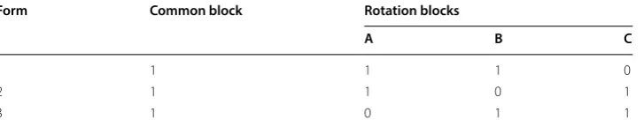
The second design we explore is the three-form design (see Graham et al. (2006)). The three-form design was implemented in PISA 2012 and is a focus of attention in this paper insofar as PISA 2012 was the first large-scale educational assessment to imple-ment a CQ matrix sampling design in their main study. In this design, we keep the com-mon block of the questionnaire scales the same as in the Adams et al. (2013) two-form design and then arrange the remaining 19 scales into the three mutually exclusive blocks A, B and C (see Table 2). The three questionnaire forms contain any of the two blocks. As Table 2 shows, form 1 contains blocks A and B, form 2 contains blocks A and C, and form 3 contains blocks B and C. In addition to the rotation blocks, each question-naire form also contains the common block. We randomly assign the three forms to the respondents. The missing percentage of the variables in the rotation blocks is 33, 17% less than the two-form design. Because all pairs of scales have observed data the correla-tions and interaccorrela-tions of the variables across rotation blocks are estimable. The assign-ment of the actual scales to the three forms can be seen in Table 3.

Table 2 Three-form design based on PISA 2012

Form Common block Rotation blocks

A B C

1 1 1 1 0

2 1 1 0 1

(8)

Partially balanced incomplete block design (Kaplan and Su 2016)

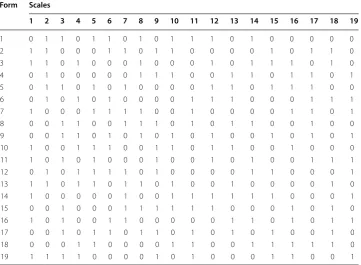
The third design that we explore is a partially balanced incomplete block design (PBIB). This design was studied in Kaplan and Su (2016) but not in the context of employing generated PVs as part of the imputation of the missing CQ variables, nor in conjunction with the SMI or MMI approaches for multiple imputation. In this design, we keep the common block of the questionnaire scales the same as in Adams et al. (2013) design and then arrange the remaining 19 scales according to a PBIB design with three associate classes (Montgomery

2012).4_{The 19 scales are assigned to 19 forms but the missing percentage for each scale is} still 50%, making it comparable to the two-form design. In our PBIB design, each cluster contains 9 or 10 scales as shown in Table 4. The scales are arranged in the 19 forms in such a fashion that all pairs of scales appear three, four or five times. For example, we see in Table 4

that scales 1 and 3 appear together 3 times, scales 1 and 2 appear together 4 times, and scales 1 and 7 appear together 5 times. We assign the common block to all 5611 respond-ents, then we randomly assign one of the 19 forms to each respondent. Respondents who get form 1 have data deleted on scale 1, 4, 7, 9, 13, and 15–19. As with the Adams et al. (2013) design, the 15 scales in the common block do not have any missing data, while the 19 scales have 50% missing data. Unlike the two-form deisgn, the PBIB design ensures that all pairs of scales have observed data.

Simulation procedures

All analyses utilized the R programming environment R Core Team (2017). Functions for generating the PVs are given in Appendix A and functions to generate CQ simula-tions are given in Appendix B. We first create the matrix sampling designs on the origi-nal CQ data. Then in order to impute the missing data and to generate the PVs, we implement the SMI and MMI approaches of Weirich et al. (2014) with slight modifica-tions. The simulation thus has six conditions in total, three matrix sampling designs by two approaches. The two approaches require us first to specify the item response model to obtain initial PVs, second impute the CQ missing data using the initial PVs, and finally Table 3 Variable assignment to blocks in the three-form design

Scale definitions can be found in Table 1

Form 1 Form 2 Form 3

Common block Common block Common block

Rotation bock 1 Rotation block 2 Rotation block 3

CARINFO SCINTACT PERSCIE

CARPREP SCINVEST RESPDEV

ENVAWARE SCSCIE SCAPPLY

INSTSCIE ENVOPT SCHANDS

JOYSCIE ENVPERC SCIEACT

SCIEFUT GENSCIE SCIEEFF

INTSCIE

4 _{Associate classes are a feature of incomplete block designs and refer to the number of times a pair of scales (or}

(9)

using the imputed CQ data as the conditioning model to impute the final PVs. The dif-ference between these two approaches is in the second step—the SMI or MMI methods for the CQ missing data. If we use SMI in the final step we generate five PVs based on the single imputed CQ. If we use MMI with five imputed CQs, in the final step 25 PVs will be generated since five PVs are generated using each of the five imputed CQs. We will then evaluate the distributions of the PVs under the six simulation conditions. The multiple PVs will also be used in the secondary analysis to explore the bias in the cor-relations between the scales and the PVs and bias in regression coefficients and their standard errors.

Calibration

In the first step, we specify the item response model. For this purpose, we use the “TAM” package (Kiefer et al. 2014) in the R software environment (R Core Team 2017) to scale the cognitive data. We implement a unidimensional one-parameter partial credit model with the ConQuest parametrization (Adams et al. 2015). The dimension is science and contains in total 102 cognitive items. Following the PISA 2006 technical report OECD (2009), we fix the item parameters at their international values and apply the sampling weights when specifying the item response model. Finally, five normally approximated PVs are generated (Chang and Stout 1993) without the conditioning model (i.e., without Table 4 Partially balanced incomplete block design for the 19 questionnaire scales

A “1” denotes the presence of the scale in the cluster, “0”, othersize

Form Scales

1 2 3 4 5 6 7 8 9 10 11 12 13 14 15 16 17 18 19

1 0 1 1 0 1 1 0 1 0 1 1 1 0 1 0 0 0 0 0

2 1 1 0 0 0 1 1 0 1 1 0 0 0 0 1 0 1 1 0

3 1 1 0 1 0 0 0 1 0 0 0 1 0 1 1 1 0 1 0

4 0 1 0 0 0 0 0 1 1 1 0 0 1 1 0 1 1 0 1

5 0 1 1 0 1 0 1 0 0 0 0 1 1 0 1 1 1 0 0

6 0 1 0 1 0 1 0 0 0 0 1 1 1 0 0 0 1 1 1

7 1 0 0 0 1 1 1 1 0 0 1 0 0 0 0 1 1 0 1

8 0 0 1 1 0 0 1 1 1 0 1 0 1 1 0 0 1 0 0

9 0 0 1 1 0 1 0 1 0 1 0 1 0 0 1 0 1 0 1

10 1 0 0 1 1 1 0 0 1 1 0 1 1 0 0 1 0 0 0

11 1 0 1 0 1 0 0 0 1 0 0 1 0 1 0 0 1 1 1

12 0 1 0 1 1 1 1 0 1 0 0 0 0 1 1 0 0 0 1

13 1 1 0 1 1 0 1 1 0 1 0 0 1 0 0 0 0 1 0

14 1 0 0 0 0 0 1 0 0 1 1 1 1 1 1 0 0 0 1

15 0 0 1 0 0 0 1 1 1 1 1 1 0 0 0 1 0 1 0

16 1 0 1 0 0 1 1 0 0 0 0 0 1 1 0 1 0 1 1

17 0 0 1 0 1 1 0 1 1 0 1 0 1 0 1 0 0 1 0

18 0 0 0 1 1 0 0 0 0 1 1 0 0 1 1 1 1 1 0

(10)

conditioning on the background information). In contrast with Weirich et al. (2014) which used the weighted maximum likelihood estimates (WLE) as proxies for individual proficiency scores to impute the CQ in the following step, we directly use the initial PVs that are generated in this step.5

Imputing questionnaire data

The second step is to impute the CQ missing data. For each matrix sampling design, we implement SMI and MMI for the CQ missing data using predictive mean matching (PMM) via the R package MICE (van Buuren and Groothuis-Oudshoorn 2010). Previous research (Kaplan and Su 2016; Kaplan and McCarty 2013) has found predictive mean matching to be quite good with respect to meeting the requirements for the validity of statistical matching and imputation set down by Räassler (2002).

Predictive mean matching

Following van Buuren (2012), (see also; Kaplan and Su (2016)), predictive mean match-ing is implemented through a fully conditional specification approach that uses a uni-variate regression model consistent with the scale of the variable with missing data to provide predicted values of the missing data given the observed data. Once a variable of interest is filled-in, that variable, along with the variables for which there is complete data, is used in a sequence to fill in another variable. Once the sequence is completed for all variables with missing data, the posterior distributions of the regression parameters are obtained via Gibbs sampling and the process is started again. The algorithm can run these sequences simultaneously M number of times obtaining M imputed data sets.

The PMM algorithm can be outlined as follows. Let Xobs be the predictors with

observed data based on n1 observations ( i=1, 2,. . .,n1 ), and let Xmiss be the predictors with missing data on a target variable y based on n0 observations ( j=1, 2,. . .,n0).

1. Obtain _βˆ_{based on}_X

obs and let σ˜2 be a draw based on the deviations

(yobs−Xobsβ)ˆ ′(yobs−Xobsβ)/˜ˆ g , where g˜ is a draw from a χ2 distribution.

2. Draw _β˜_{= ˆ}_β_{+ ˜}_σz˜1V1/2 , where V1/2 is the square root of the Cholesky

decomposi-tion of the cross-products matrix S=X_obs′ Xobs , and z1 is a p-dimensional vector of N(0, 1) random variates.

3. Calculate _δ(˜ _i_,_j₎_{= |}_X

obs,[i]βˆ−Xmiss,[j]β|˜ ; i=1, 2,. . .,n1 , j=1, 2,. . .,n0.

4. Construct n0 sets Wj , each containing d candidate donors from yobs , such that

dδ(˜i,j) is minimum. Break ties randomly.

5. Randomly draw one donor ij from Wj for j=1, 2,. . .,n0.

6. Impute y˜j=yij , for j=1, 2,. . .,n0.

The imputation model includes all 34 scales, school ID, cluster ID and the five initial PVs that were generated in the first step. The interaction terms between gender and all the other scales were also included and passive imputation was used. Passive imputation is a method for imputing functions (e.g. transformations or interactions) among incomplete

(11)

variables when both the original and transformed variables are needed in the imputation models. For PV generation, the original variables and interactions are required and thus missing on each requires passive imputation (see van Buuren (2012), for more informa-tion). For the single imputation, we obtain one complete CQ data set and for the multi-ple imputations we obtain five commulti-plete CQ data sets.

Generating final PVs

In the third step, we generate the final PVs conditioning on the imputed CQ data set. The item response model is the same as the calibration step except for conditioning on all the CQ variables in Table 1. Five normally approximated PVs are generated using one complete CQ data set. Thus for the MMI approach, we generate 25 PVs using the five imputed data sets. The generated PVs are all placed on the PISA scale (OECD 2009, p. 246). The final PVs are then used in the subsequent analyses.

Analysis

In the analysis step, we are interested in (1) how the distributions of the PVs under the six simulation conditions differ from the distributions of the PVs that are generated from the original questionnaire data; (2) how the correlations of CQ variables under the six conditions differ from the original questionnaire data; and (3) how regression coefficients differ across the six conditions compared to regression results from the original data.

To assess the distributions of PVs under the three planned missing data designs and two imputation approaches, we use the PVs conditioning on the original CQ data as the baseline comparison. The procedure for generating the PVs is the same as in the previous step: five PVs are generated by conditioning on the original data with all scales shown in Table 1. We calculate the mean and the standard errors of the PVs. The mean of PVs is simply the average across the five or 25 PVs. The standard errors under the SMI approach is pooled using Rubin’s rules (1987). The standard error under the MMI approach is pooled using the modified combining rules (Rubin 2003). In addition, we also conduct Kolmogorov Smirnov tests to compare the distributions of PVs.

Modified combining rules

Following Rubin (2003), the modified combining rules are as follows: let Q rep-resent a quantity of interest, let _Qˆ(m,n)_{represent the mean estimate of the}_m_th_PV

(m=1, 2,. . .M) , and let n=1, 2,. . .N be the nth imputation of the CQ. Then,

is the overall average PV across imputations and nests. A vector of N mean estimates over the M PVs within each nest can be formed as

(1)

¯

Q= 1

NM

N

n=1 M

m=1 ˆ

(12)

Let _U¯_{represent the average of the variance estimates over the}_N_{nests and}_M imputa-tions, written as

Let MS(b)_{be the between-nest mean square,}

and let MS(w) be the within-nest mean square

Then, as shown by Rubin (2003), the total imputation variance (Q− ¯Q) can be estimated by

We calculate the pairwise correlations among all CQ scales, including those between CQ variables and PVs. Because there are multiply imputed CQ data sets under MMI approach, we take the average of the correlations across the data sets. Then, the bias in correlations is calculated as the difference between the averaged correlations and the true correlations from the original data. As a baseline for comparison, we use the corre-lations from the original CQ data.

To assess the regression coefficients under the six conditions, we conduct multiple regression analyses by regressing the multiple PVs on the selected scales. Note that we intentionally chose an analytic model which is simpler than the model that is used to generate PVs to reflect the realistic situation in which the researcher may not be aware of the full set of variables that were used in the conditioning model and is instead focusing his/her attention on a small set of theoretically motivated variables.

In the regression analysis, student sampling weights are added to reflect the complex sampling design of PISA 2006 (see OECD (2009), for more details). We then pool the 5 or 25 regression analyses according to Rubin’s rules (1987; 2003, respectively). To have a baseline to compare to, we use the coefficients and standard errors from the regres-sion analysis based on the original data (with the same regresregres-sion model). We calculate the standardized bias of the coefficient estimates as the difference between the pooled estimates and the counterpart estimates based on the original data, standardized by the standard deviation of the outcome variable. We calculate the ratio of variances as the

(2)

¯

Qn= 1

M M

m=1 ˆ

Q(n,m).

(3)

¯

U = 1

NM N n=1 M m=1 U(n,m).

(4) MS(b)= M

N−1 N

n=1

(Q¯n− ¯Q)2,

(5)

MS(w)= 1

N(M−1)

N

n=1 M

m=1

(Q¯(n,m)− ¯Qm)2.

(6)

T = ¯U+ 1

M

1+ 1

N

MS(w)+

1+ 1

M

(13)

squared pooled standard errors under each condition over the squared standard errors from the original data. It is expected that the ratio of the variances should be greater than one, since the standard errors under the six conditions must reflect the uncertainty due to the generation of PVs or imputation of the CQ data. The magnitude of the ratio depends on the choice of the design and the uncertainty from the generation of PVs or imputation of the CQ.

Results

In this section we first present the results of the marginal distributions of the PVs. This is followed by a presentation of the correlation bias. Finally, we present the results of regression analysis. We show that the marginal distributions of the PVs under the six simulation conditions do not differ from those that are generated from the original questionnaire data. The correlations among CQ variables differ across designs but not the methods. The estimates of regression coefficients differ across the design and the methods.

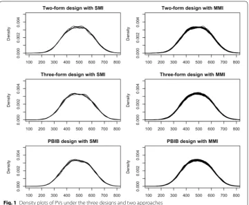
Marginal PV distributions

The means and standard errors of PVs for the original data and under the six conditions (three designs × two imputation approaches) are presented in Table 5 and plots of the densities of PVs are shown in Fig. 1. Table 6 shows the p values of Kolmogorov–Smirnov tests when comparing the first PV under each of the six simulation conditions to the first PV of the baseline condition. We observe that the means of the marginal distribu-tions are virtually identical across the designs and the methods. This result is consistent with Kaplan and Su (2016). However, in this case, we do observe sizably larger pooled Table 5 Pooled mean and standard error of PVs

Design Approach Pooled mean Pooled SE

Original design 489.004 216.964

Two-form design SMI 489.111 141.671

MMI 489.105 355.791

Three-form design SMI 489.110 120.215

MMI 489.253 388.075

PBIB SMI 489.070 182.998

MMI 489.228 322.087

Table 6 Kolmogorov–Smirnov tests

The Kolmogorov–Smirnov test compares the distribution of the first PV from each simulation condition (6 in total = 2 approaches × 3 designs) with the first PV from the original complete data (H0: the two sample distributions are drawn from the same distribution)

Design p value

Two-form SMI vs. original 0.79

Two-form MMI vs. original 0.94

Three-form SMI vs. original 0.80

Three-form MMI vs. original 0.93

PBIB SMI vs. original 0.86

(14)

standard errors from MMI versus SMI across designs. This is not unexpected insofar as MMI accounts for greater uncertainty in the imputation process. Interestingly, because the single imputation approach does not take full account of the uncertainty of the planned missing data, the standard errors from SMI method are smaller than from the original design. We also notice that the pooled standard errors are different across the designs due to the planned missing data patterns. The Kolmogorov-Smirnov test results show that the distribution of the first PVs are not significantly different from the PV of the original data.

Correlation bias

For the SMI and MMI approaches under each planned missing data design we calculate the pairwise correlations among all CQ scales, including those between CQ variables and PVs. In order to compute the bias in correlations, we use the correlations of the original CQ as the true correlation values. The bias in correlations is calculated as the difference between the averaged correlations across multiple imputed data sets and the true correlations from the original data.

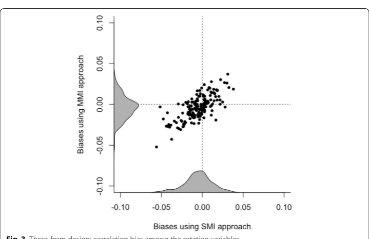
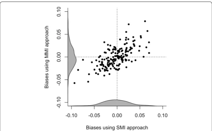
Figures 2, 3, and 4 plot the correlation biases among CQ variables under MMI against the correlation bias for SMI across the two-form, three-form, and PBIB designs, respectively. We observe that the correlation bias is substantially lower for the three-form design implemented in PISA 2012, compared to the two-form and PBIB design. We find the PBIB design to perform better with respect to correlation

(15)

bias compared to the two-form design, even though the overall amount of missing data for these two designs are the same. Little difference is found between the SMI or MMI approaches with respect to correlation bias across the planned missing data designs. For the correlations between CQ variables and PVs, we found no difference across the designs and the methods.6

Fig. 2 Two-form design: correlation bias among the rotation variables

Fig. 3 Three-form design: correlation bias among the rotation variables.

(16)

Regression analysis

Figure 5 presents the standardized bias in the estimated regression coefficients across the designs for SMI and MMI respectively. The scales to the left of the vertical lines in each plot are the variables in the common block. In Fig. 5 we observe for both SMI and MMI methods, less bias is found for scales in the common block compared to scales in the rotated blocks because variables in the common block are not part of the planned missing data. As with the correlation bias results, the three-form design implemented in PISA 2012 shows the least amount of bias in the regression coefficients. For the SMI method, all variables in three-form design have the standardized biases within 0.08 in absolute value, followed by 93% of the variables in PBIB design and 87% of the variables in the two-form design. For the MMI method, the three-form design and PBIB design have standardized biases for all variables within 0.08 in absolute value, and only 90% in the two-form design. In addition the two-form design produces several more extreme biased coefficients, as can be seen in the scales SCINTACT, SCAPPLY, and SCHANDS.

Figure 6 presents the results of standard errors of the regression coefficients for the SMI and MMI methods. The plots show the ratio of the squared standard errors of regression coefficients from the three rotation designs over the original design. First, we observe almost all the ratios are larger than one as expected because the standard errors from the rotation designs have to account for the uncertainty due to missing data, while the original design does not contain any missing data, resulting in smaller stand-ard errors. Second, we observe that the ratios of variables are much larger using MMI method than SMI method. This is also expected because multiple imputation results in larger standard errors than the single imputation. Third, for the scales in the common block, the ratios are much closer to one than the scales in rotation blocks because there is no missing data in the common block scales. Finally, across the designs, we observe that the ratios from the three-form design are smaller than those for the PBIB design and the two-form design. For the SMI method, none of the standard errors from the

(17)

three-form design is 100% larger than from the original design, however 30% of the ratios in the PBIB design and 10% in the two-form design are larger than two. For the MMI method, the two-form design produces much larger standard errors than the other two designs, with 50% standard errors at least two times larger than the original design, followed by 47% in the PBIB design and 10% in the three-form design.7

Overall, due to less missing data, the three-form design produces less bias in the regression coefficients and smaller standard errors than the PBIB design. The PBIB design still performs better than the two-form design even though they have the same amount of missing data. This is because the PBIB design allows all pairs of scales to have data and so the correlations among all pairs of scales can be preserved, which is not the case with the two-form design.

Fig. 5 Regression coefficient estimates under SMI and MMI approaches

Fig. 6 Standard errors of the regression coefficients under SMI and MMI approaches

(18)

Conclusions

This paper expanded on earlier work by Weirich et al. (2014) in two ways. First, we showed that it is possible to use PVs simply and directly via nested multiple imputa-tion. Consistent with the results of Weirich et al. (2014), we found that nested mul-tiple imputation with PVs provides considerable bias reduction as expected under the framework of congenial missing data models. Also, consistent with Weirich et al. (2014), our findings showed relatively similar results for SMI and MMI. It should be pointed out that it is possible to implement a procedure that combines the PVs and CQ in one algorithm for simultaneous imputation (see Aßman et al. (2015)). The approach of Aßman et al. (2015) was studied under general missing data in the CQ but should be compared to the SMI and MMI approaches in the context of planned missing data in future studies. Second, we showed that the three-form design as implemented in PISA 2012 performed better in terms of correlation and regression bias reduction compared to the PBIB design examined in Kaplan and Su (2016) and the two-form design of Adams et al. (2013). The bias reduction in the partial bal-anced incomplete design is still better than what is achieved under the two-form design with the same overall amount of missing data. Further studies on investi-gating the variations of incomplete block designs for CQs are still needed because there are many other design possibilities (e.g., amount of missing data, missing-ness on items within scales etc.) that may be well-suited to large-scale educational assessments.

To conclude, the cumulative research on multiple imputation methods (Schafer and Graham 2002; Reiter and Raghunathan 2007; Harel 2007; Rubin 2003) applied to context questionnaires (Aßman et al. 2015; Adams et al. 2013; Kaplan and Su 2016; Weirich et al.

2014), shows relatively minimal impact on the marginal distributions of PVs and the joint relations of PVs with context questionnaire scales. The present study adds to the lit-erature by comparing three planned missing data designs under two approaches to mul-tiple imputation. Given that a common concern facing most national and international large-scale assessments is the desire to present as much content as possible without over-burdening the participants in the survey and furthermore given increased interest in the so-called “non-cognitive” outcomes of education we argue that the approach to questionnaire matrix sampling and imputation described in this paper should be given serious consideration.

Authors’ contributions

DK conceptualized the study and guided the design of the study, the statistical analysis, and contributed to drafting the manuscript. DS contributed to the design and development of the the software to conduct the analysis, carried out the analysis as well as contributed to drafting the manuscript. Both authors read and approved the final manuscript.

Acknowledgements

Not applicable.

Competing interests

The authors declare that they have no competing interests.

Availability of data and materials

The datasets supporting the conclusions of this article are available at http://bise.wceru w.org/index .html. The software supporting used to support the conclusions of this article are included within the article and also available at http://bise. wceru w.org/index .html.

Funding

(19)

Appendix A

# :::::::::::::::::::::::::::::::::::::::::::::: # :::::::::Functions for PV generation:::::::::: # ::::::::::::::::::::::::::::::::::::::::::::::

## These are the functions and data that need to run before simulations

library(foreign) library(TAM) library(mice)

setwd('~/Dropbox/PISA')

# variable names

var.c <- c('PROGN', 'ST01Q01', 'AGE', 'ST04Q01', 'BMMJ', 'BFMJ', 'BSMJ', 'MISCED', 'FISCED', 'IMMIG', 'ST11Q04', 'ST12Q01', 'DEFFORT',

'CULTPOSS', 'HEDRES', 'WEALTH')

var1 <- c('CARINFO', 'CARPREP', 'ENVAWARE', 'INSTSCIE', 'JOYSCIE', 'SCIEFUT', 'SCINTACT', 'SCINVEST', 'SCSCIE')

var2 <- c('ENVOPT', 'ENVPERC', 'GENSCIE', 'INTSCIE',

'PERSCIE', 'RESPDEV', 'SCAPPLY', 'SCHANDS','SCIEACT', 'SCIEEFF')

var0 <- c('AGE', 'ST04Q01', 'BMMJ', 'BFMJ', 'BSMJ', 'IMMIG', 'DEFFORT', 'CULTPOSS', 'HEDRES', 'WEALTH', var1, var2)

# Load raw data

std <- read.spss('student_context_USA06.sav', to.data.frame = T) # questionnaire

cog <- read.spss('COG_USA06.sav', to.data.frame = T)

names(cog) dim(std) names(std)

# attach bookid in std

cog <- cog[order(as.numeric(cog$STIDSTD)), ] sum(cog$STIDSTD != std$STIDSTD)

std$BOOKID <- cog$BOOKID

#transform to numeric

cog1 <- as.data.frame(sapply(cog, as.numeric) - 1) dim(cog1)

# missing checking cog2 <- cog1[, 8:275]

colnames(cog2)[sapply(cog2, function(x) sum(is.na(x)) == 5611)] ## no reading cognitive test for USA

sapply(cog2, function(x) sum(is.na(x)))

# Load Original CQ

load('con_origin06_pmm_m1.RData') # original CQ impputed (no item missing)

sapply(con.or, function(x) sum(is.na(x)))

# Load rotated PBIB CQ

load(file = 'PISA06_CQ_PBIB.RData')

sapply(con.pbib, function(x) sum(is.na(x))) # no item missing PBIB CQ

# load rotated Adams CQ

load(file = 'PISA06_rotated_Adams.RData') # no item missing Adams CQ sapply(con.adam, function(x) sum(is.na(x)))

# load rotated 3form CQ

(20)

# --- imp.pv ---

---imp.pv <- function(conpv, m){

# imp.1pv ... impute the rotated CQ with 1PV with sex interaction, return a list of 5 datasets

# conpv ... data frame with CQ + 1PV # m ...number of multiple imputations

# attach interactions with sex

var.r <- c('CARINFO', 'CARPREP', 'ENVAWARE', 'INSTSCIE', 'JOYSCIE',

'SCIEFUT', 'SCINTACT', 'SCINVEST', 'SCSCIE',

'ENVOPT', 'ENVPERC', 'GENSCIE', 'INTSCIE', 'PERSCIE', 'RESPDEV', 'SCAPPLY', 'SCHANDS','SCIEACT', 'SCIEEFF')

nam.int <- paste("ST04Q01.1.", var.r, sep = '')

int <- matrix(NA, nrow = nrow(conpv), ncol = length(var.r)) colnames(int) <- nam.int

conpvi <- cbind(conpv, int)

# multiple imputation

ini <- mice(conpvi, maxit = 0, pri = F) meth <- ini$meth

meth[nam.int] <- paste('~I(ST04Q01.1*', var.r, ')', sep = '') meth[colnames(conpv)] <- rep('fastpmm', ncol(conpv)) pred <- ini$pred

pred[var.r, nam.int] <- 0

pred[, c('STIDSTD', 'BOOKID')] <- 0

out.imp <- mice(conpvi, pred = pred, meth = meth, m = m)

# extract imputed dataset

conpv.imp <- lapply(1:m, complete, x = out.imp) invisible(conpv.imp)

}

# --- PV ---

---PV.imp <- function(con.imp, w) {

# PV... generate 5 PVs for one conditional questionnaire with no missing data (return matrix of 5 pvs)

# con.imp ... imputed CQ with no missng data

# ******* Prepare conditioning variables for original con data ***** # ::::: Direct conditioning variables ::::

# booklet id

table(con.imp$BOOKID)

con.imp$BOOKID <- relevel(factor(con.imp$BOOKID), ref = '13') con.imp$BOOKID <- relevel(factor(con.imp$BOOKID), ref = '12')

contrasts(con.imp$BOOKID) <- contr.sum(13); contrasts(con.imp$BOOKID) # deviation coding

# school

max(table(con.imp$SCHOOLID)) # 00070 is the largest school

con.imp$SCHOOLID <- relevel(factor(con.imp$SCHOOLID), ref = '00070') # direct conditioning variables

dvar <- con.imp[, c('BOOKID', 'SCHOOLID')]

# ::::: combine direct and indirect conditioning variables :::::: var.c <- c('PROGN', 'ST01Q01', 'AGE', 'ST04Q01', 'BMMJ', 'BFMJ', 'BSMJ', 'MISCED', 'FISCED', 'IMMIG', 'ST11Q04', 'ST12Q01', 'DEFFORT',

'CULTPOSS', 'HEDRES', 'WEALTH')

var1 <- c('CARINFO', 'CARPREP', 'ENVAWARE', 'INSTSCIE', 'JOYSCIE', 'SCIEFUT', 'SCINTACT', 'SCINVEST', 'SCSCIE')

var2 <- c('ENVOPT', 'ENVPERC', 'GENSCIE', 'INTSCIE',

'PERSCIE', 'RESPDEV', 'SCAPPLY', 'SCHANDS','SCIEACT', 'SCIEEFF')

(21)

## no missing ensures con.mat the same row dim as con.var con.mat <- model.matrix(~., con.var)[, -1]

con.mat <- con.mat[, apply(con.mat, 2, function(x) length(table(x))) != 1] # get rid of no variance varibales

# ****** Unidimensional 1PL PV generation ***** # science dimention parameters

par3 <- read.table('06par3.txt') nam.sc3 <- names(cog2)[c(77:179)] sum(par3$V1 != nam.sc3)

par.st3 <- par3[par3$V3 < 3, 3] # extract from the second column data the step parameter

xsi3 <- c(par3[, 2], par.st3)

xsi3 <- cbind(seq(1,length(xsi3)), xsi3) # scaling

out <- tam.mml(resp = cog2[, nam.sc3], xsi.fixed = xsi3, Y = con.mat, irtmodel = 'PCM2', pweights = w)

pv <- tam.pv(out, nplausible = 5 , ntheta = 1000, normal.approx=TRUE)

# Standardize PV

pv <- cbind(pv$pv$PV1.Dim1, pv$pv$PV2.Dim1, pv$pv$PV3.Dim1, pv$pv$PV4.Dim1, pv$pv$PV5.Dim1)

pv <- apply(pv, 2, function(x) ((x - 0.1797) / 1.0724) * 100 + 500) colnames(pv) <- c('PV1', 'PV2', 'PV3', 'PV4' ,'PV5')

invisible(pv) }

# --- PV ---

---# --- pool regression ---

---PVreg.or <- function(pv, con, var, w){

# PVreg.or ... for CQ no missingness, pool the regression results (output is a list of pooled results)

# pv ... final PVs, output from PV.imp() # con ... conditional questionnaire data # var ... variables in the regression model # w ... sampling weights in lm

# ::::::: pool regression :::::::::: conpv <- data.frame(cbind(con, pv))

out1 <- lm(conpv$PV1 ~ . , data = conpv[, var], weights = w) out2 <- lm(conpv$PV2 ~ . , data = conpv[, var], weights = w) out3 <- lm(conpv$PV3 ~ . , data = conpv[, var], weights = w) out4 <- lm(conpv$PV4 ~ . , data = conpv[, var], weights = w) out5 <- lm(conpv$PV5 ~ . , data = conpv[, var], weights = w)

outp <- as.mira(list(out1, out2, out3, out4, out5)) out <- summary(pool(outp))

R2 <- c(summary(out1)$r.squared, summary(out2)$r.squared, summary(out3)$r.squared,

summary(out4)$r.squared, summary(out5)$r.squared) R2.p <- pool.r.squared(outp)

list(out, R2 = R2, Pool.R2 = R2.p) }

sub.pool <- function(conpv, var, w){

# sub.pool... put together lm results of single imputed CQ (regressed on 5 PVs), return a list of lm output

# conpv ... one imputed CQ with corresponding 5 PVs # var ... variables in the regression model

# w ... sampling weights in lm

(22)

outp <- list(out1, out2, out3, out4, out5) invisible(outp)

}

PVreg.rot <- function(conpv.list, var, w){

# PVreg.or ... for rotated CQ, pool the regression results (output is a matrix of pooled results) using sub.pool()

# conpv.list ... a list of multiple imputed CQ with 5 PVs # var ... variables in the regression model

# w ... sampling weights in lm

# ::::::: pool regression ::::::::::

outl <- lapply(conpv.list, sub.pool, var = var, w = w)

outp<- as.mira(list(outl[[1]][[1]], outl[[1]][[2]], outl[[1]] [[3]], outl[[1]][[4]], outl[[1]][[5]],

outl[[2]][[1]], outl[[2]][[2]], outl[[2]] [[3]], outl[[2]][[4]], outl[[2]][[5]],

outl[[5]][[1]], outl[[5]][[2]], outl[[5]] [[3]], outl[[5]][[4]], outl[[5]][[5]]))

out <- summary(pool(outp)) R2.p <- pool.r.squared(outp) list(out, Pool.R2 = R2.p) }

(23)

---Appendix B

# :::::::::::::::::::::::::::::::::::::::::::::::::::: # :::::::::: Secondary analysis on imputed CQs ::::::: # ::::::::::::::::::::::::::::::::::::::::::::::::::::

# please run the function file first!

library(foreign) library(TAM) library(mice)

setwd('Dropbox/PISA')

# =========================== SMI MMI (with 5pvs) save results ===========================

# SMI MMI and three designs (with 5pvs in imputation)

# :::::::::::::: scaling and generate the original 5pv to put in imputation :::::::::::::

# science dimention parameters par3 <- read.table('06par3.txt') nam.sc3 <- names(cog2)[c(77:179)] sum(par3$V1 != nam.sc3)

par.st3 <- par3[par3$V3 < 3, 3] # extract from the second column data the step parameter

xsi3 <- c(par3[, 2], par.st3)

xsi3 <- cbind(seq(1,length(xsi3)), xsi3) # scaling

out <- tam.mml(resp = cog2[, nam.sc3], xsi.fixed = xsi3, irtmodel = 'PCM2', pweights = std$W_FSTUWT)

# PV

pv <- tam.pv(out, nplausible = 5 , ntheta = 1000, normal.approx=TRUE) # Standardize PV

pv <- cbind(pv$pv$PV1.Dim1, pv$pv$PV2.Dim1, pv$pv$PV3.Dim1, pv$pv$PV4.Dim1, pv$pv$PV5.Dim1)

pv <- apply(pv, 2, function(x) ((x - 0.1797) / 1.0724) * 100 + 500) colnames(pv) <- c('PV1', 'PV2', 'PV3', 'PV4' ,'PV5')

# :::::::::::::::: origin ::::::::::::::::

outo <- PVreg.or(pv, con.or, var0, w = std$W_FSTUWT)

# :::::::::::::::: PBIB :::::::::::::::: # combine rotated CQ with pv5

conpv.pbib5 <- cbind(con.pbib, pv) # 5 PVs

# 2. imput rotated CQ with pv5

imp.pbib1 <- imp.pv(conpv.pbib5, m = 1) imp.pbib5 <- imp.pv(conpv.pbib5, m = 5)

# 3. Generate 5 PVs for each

pv.b1 <- lapply(imp.pbib1, PV.imp, w = std$W_FSTUWT) pv.b5 <- lapply(imp.pbib5, PV.imp, w = std$W_FSTUWT)

# combine each imputed CQ with corresponding PV

expv5 <- c('PV1','PV2','PV3','PV4','PV5') # exclude the 5 cheap pv

imp.b1 <- cbind(imp.pbib1[[1]], pv.b1[[1]]) imp.b5 <- list()

for(i in 1:5){imp.b5 [[i]] <- cbind(imp.pbib5[[i]][, !is.element(colnames(imp.pbib5[[1]]), expv5)], pv.b5[[i]])}

# 4. pool regression # SMI (1st dataset * 5PVs)

outb1 <- PVreg.or(pv.b1[[1]], imp.b1, var0, std$W_FSTUWT) #MMI (5datasets* 5PVs for each)

(24)

# :::::::::::::::: Adams :::::::::::::::: # combine rotated CQ with pv5

conpv.adam5 <- cbind(con.adam, pv) # 5 PVs

# 2. imput rotated CQ with pv5

imp.adam1 <- imp.pv(conpv.adam5, m = 1) imp.adam5 <- imp.pv(conpv.adam5, m = 5)

pv.a1 <- lapply(imp.adam1, PV.imp, w = std$W_FSTUWT) pv.a5 <- lapply(imp.adam5, PV.imp, w = std$W_FSTUWT)

# combine each imputed CQ with corresponding CQ

expv5 <- c('PV1','PV2','PV3','PV4','PV5') # exclude the 5 cheap pv

# combine each imputed CQ with corresponding PV imp.a1 <- cbind(imp.adam1[[1]], pv.a1[[1]]) imp.a5 <- list()

for(i in 1:5){imp.a5 [[i]] <- cbind(imp.adam5[[i]][, !is.element(colnames(imp.adam5[[1]]), expv5)], pv.a5[[i]])}

outa1 <- PVreg.or(pv.a1[[1]], imp.a1, var0, std$W_FSTUWT) #MMI (5datasets* 5PVs for each)

outa5 <- PVreg.rot(imp.a5, var0, w = std$W_FSTUWT)

# :::::::::::::::: 3form :::::::::::::::: # combine rotated CQ with pv5

conpv.f5 <- cbind(con.f3, pv)

# 2. imput rotated CQ with pv5 imp.3f1 <- imp.pv(conpv.f5, m = 1) imp.3f5 <- imp.pv(conpv.f5, m = 5)

pv.f1 <- lapply(imp.3f1, PV.imp, w = std$W_FSTUWT) pv.f5 <- lapply(imp.3f5, PV.imp, w = std$W_FSTUWT)

# combine each imputed CQ with corresponding CQ imp.f1 <- cbind(imp.3f1[[1]], pv.a1[[1]]) imp.f5 <- list()

for(i in 1:5){imp.f5 [[i]] <- cbind(imp.3f5[[i]][, !is.element(colnames(imp.3f5[[1]]), expv5)], pv.f5[[i]])}

outf1 <- PVreg.or(pv.f1[[1]], imp.f1, var0, std$W_FSTUWT) #MMI (5datasets* 5PVs for each)

outf5 <- PVreg.rot(imp.f5, var0, w = std$W_FSTUWT)

# save MMI results

save(pv, outo, imp.pbib1, imp.pbib5, pv.b1, pv.b5,

imp.adam1, imp.adam5, pv.a1, pv.a5, imp.3f1, imp.3f5, pv.f1, pv.f5, file = "Results61.Rdata")

# ================================= read results ==========================================

(25)

# combine each imputed CQ with corresponding PV

expv5 <- c('PV1','PV2','PV3','PV4','PV5') # exclude the 5 cheap pv imp.b1 <- cbind(imp.pbib1[[1]], pv.b1[[1]])

imp.b5 <- list()

for(i in 1:5){imp.b5 [[i]] <- cbind(imp.pbib5[[i]][, !is.element(colnames(imp.pbib5[[1]]), expv5)], pv.b5[[i]])}

imp.a1 <- cbind(imp.adam1[[1]], pv.a1[[1]]) imp.a5 <- list()

for(i in 1:5){imp.a5 [[i]] <- cbind(imp.adam5[[i]][, !is.element(colnames(imp.adam5[[1]]), expv5)], pv.a5[[i]])}

imp.f1 <- cbind(imp.3f1[[1]], pv.f1[[1]]) imp.f5 <- list()

for(i in 1:5){imp.f5 [[i]] <- cbind(imp.3f5[[i]][, !is.element(colnames(imp.3f5[[1]]), expv5)], pv.f5[[i]])}

# pool regression

outb1 <- PVreg.or(pv.b1[[1]], imp.b1, var0, std$W_FSTUWT) outb5 <- PVreg.rot(imp.b5, var0, w = std$W_FSTUWT)

outa1 <- PVreg.or(pv.a1[[1]], imp.a1, var0, std$W_FSTUWT)

outa5 <- PVreg.rot(imp.a5, var0, w = std$W_FSTUWT)

outf1 <- PVreg.or(pv.f1[[1]], imp.f1, var0, std$W_FSTUWT) outf5 <- PVreg.rot(imp.f5, var0, w = std$W_FSTUWT)

# ================================= Ploting PV distributions ==========================================

lapply(pv.b1, range) par(mfrow = c(3,2)) par(mar = c(5,4,2,1))

plot(0, pch='', xlim = c(100, 800), ylim = c(0, 0.005), xlab = 'PVs', ylab = 'Density',

main = 'Two-form design with SMI') for (i in 1:5){

lines(density(pv.a1[[1]][, i])) }

main = 'Two-form design with MMI') for (i in 1:5){

for(j in 1:5){

lines(density(pv.a5[[i]][, j])) }

}

main = 'Three-form design dewith SMI') for (i in 1:5){

lines(density(pv.f1[[1]][, i])) }

main = 'Three-form design with MMI') for (i in 1:5){

for(j in 1:5){

lines(density(pv.f5[[i]][, j])) }

}

main = 'PBIB design with SMI') for (i in 1:5){

(26)

main = 'PBIB design with MMI') for (i in 1:5){

for(j in 1:5){

lines(density(pv.b5[[i]][, j])) }

}

# Table of pooled mean and se matpv <- pv.b1[[1]]

lpv <-pv.b5

pool.mi <- function(matpv){

# pool the standard error for single imputation with 5 PVs, input the matrix of 5 PVs

m.g <- apply(matpv, 2, mean) # group mean m1 <- mean(m.g) #single mean

var.g <- apply(matpv, 2, var) var1 <- mean(var.g) #single variance

var.between <- sum((var.g - var1)^2) / (length(var.g) - 1) var.total <- var1 + (1+1/length(var.g))*var.between

c(m1, sqrt(var.total)) }

pool.nmi <- function(lpv){

# pool the standard error for nested multiple imputation with 25 PVs, input the list of 5 matrix PVs

matpv <- cbind(lpv[[1]], lpv[[2]],lpv[[3]],lpv[[4]],lpv[[5]]) n.nest <- length(lpv)

n.group <- ncol(lpv[[1]])

m.g <- apply(matpv, 2, mean) # group mean m1 <- mean(m.g) #single mean

matm.g <- matrix(m.g, nrow = n.group, byrow = T) m.n <- apply(matm.g, 1, mean)

var.g <- apply(matpv, 2, var) var1 <- mean(var.g) #single variance

matvar.g <- matrix(var.g, nrow = n.group, byrow = T) var.n <- apply(matvar.g, 1, mean)

var.between <- sum((var.n - var1)^2) * (n.group/(n.nest - 1)) var.within <- (1/n.nest*(n.group-1)) * sum(sum((var.g - rep(var.n, each = n.group))^2))

var.total <- var1 + (1/n.group)*(1+1/n.nest)*var.between + (1-1/n.group)*var.within

c(m1, sqrt(var.total)) }

o.pv <- pool.mi(pv)

b1.pv <- pool.mi(pv.b1[[1]]) b5.pv <- pool.nmi(pv.b5)

a1.pv <- pool.mi(pv.a1[[1]]) a5.pv <- pool.nmi(pv.a5)

(27)

tab.pv <- round(rbind(o.pv, b1.pv, b5.pv, a1.pv, a5.pv, f1.pv, f5.pv), 3)

write.csv(tab.pv, "results6_pvpooled.csv")

# k-s test

ks.test(pv[, 1], pv.a1[[1]][, 1]) ks.test(pv[, 1], pv.a5[[1]][, 1]) ks.test(pv[, 1], pv.b1[[1]][, 1]) ks.test(pv[, 1], pv.b5[[1]][, 1]) ks.test(pv[, 1], pv.f1[[1]][, 1]) ks.test(pv[, 1], pv.f5[[1]][, 1])

# ================================= Plot correlation ==========================================

# pool correlation between cq and pv pool.cor1 <- function(imp1, pv1, var0){

# average correlations for 5 PVs(list)and 1 imputed data set(list) imp.b0 <- sapply(imp1[[1]][, var0], as.numeric)

corb <- apply(pv1[[1]], 2, function(x) cor(x,imp.b0)) apply(corb, 1, mean)

}

pool.cor5 <- function(imp5, pv5, var0){

# average correlations for 25 PVs and 5 data sets correspondingly

imp.b0 <- list()

for(i in 1:5){imp.b0[[i]] <- imp5[[i]][, var0]} # extract variables data only

for(i in 1:5){imp.b0[[i]] <- sapply(imp.b0[[i]], as.numeric)} # to numeric

corb <- list() mcorb <- list() for(i in 1:5){

corb[[i]] <- apply(pv5[[i]], 2, function(x) cor(x,imp.b0[[i]])) # correlation of each data set with corresponding PVs

mcorb[[i]] <- apply(corb[[i]], 1, mean) # avrage correlations mcorb <- cbind(mcorb[[1]], mcorb[[2]], mcorb[[3]], mcorb[[4]], mcorb[[5]]) #combine averaged correlations from 5 data sets apply(mcorb, 1, mean) # average across 5 data sets }

}

# pool correlation between cq acor1 <- function(imp1, var0){

# correlations of CQ variables in 1 imputed data set(list) imp.b0 <- sapply(imp1[[1]][, var0], as.numeric)

cor(imp.b0) }

pool.acor5 <- function(imp5, var0){

# average correlations of CQ variables in 5 data sets correspondingly

imp.b0 <- list()

for(i in 1:5){imp.b0[[i]] <- imp5[[i]][, var0]} # extract variables data only

for(i in 1:5){imp.b0[[i]] <- sapply(imp.b0[[i]], as.numeric)} # to numeric

corb <- list() mcorb <- list() for(i in 1:5){

corb[[i]] <- cor(imp.b0[[i]])} # correlation of each data set acorb <- array(unlist(corb), dim = c(nrow(corb[[1]]), ncol(corb[[1]]), length(corb))) # to array

(28)

# original CQ

coror <- pool.cor1(list(con.or), list(pv), var0) acoror <- acor1(list(con.or), c(var1, var2))

# PBIB

corb1 <- pool.cor1(imp.pbib1, pv.b1, var0) corb5 <- pool.cor1(imp.pbib5, pv.b5, var0) acorb1 <- acor1(imp.pbib1, c(var1, var2)) acorb5 <- pool.acor5(imp.pbib5, c(var1, var2))

# Adams

cora1 <- pool.cor1(imp.adam1, pv.a1, var0) cora5 <- pool.cor1(imp.adam5, pv.a5, var0) acora1 <- acor1(imp.adam1, c(var1, var2)) acora5 <- pool.acor5(imp.adam5, c(var1, var2))

# 3form

corf1 <- pool.cor1(imp.3f1, pv.f1, var0) corf5 <- pool.cor1(imp.3f5, pv.f5, var0) acorf1 <- acor1(imp.3f1, c(var1, var2)) acorf5 <- pool.acor5(imp.3f5, c(var1, var2)) # :::::: table :::::::

tab.cor <- round(cbind(coror, corb1, corb5, cora1, cora5, corf1, corf5), 3)

write.csv(tab.cor, "results6_corpooled.csv")

tab.acor <- round(rbind(acorb1-acoror, acorb5-acoror, acora1-acoror, acora5-acoror, acorf1-acoror, acorf5-acoror), 3)

write.csv(tab.acor, "results6_acorpooled.csv")

# :::::::: plot ::::::::

# Plot bias in cor of PBIB vs Adams on PVs bcor5 <- corb5-coror

bcor1 <- corb1-coror acor5 <- cora5-coror acor1 <- cora1-coror fcor5 <- corf5-coror fcor1 <- corf1-coror

round(cbind(bcor5, acor5, fcor5, bcor1, acor1, fcor1), 2)

bcor5 <- (acorb5-acoror)[upper.tri(acoror)] bcor1 <- (acorb1-acoror)[upper.tri(acoror)] acor5 <- (acora5-acoror)[upper.tri(acoror)] acor1 <- (acora1-acoror)[upper.tri(acoror)] fcor5 <- (acorf5-acoror)[upper.tri(acoror)] fcor1 <- (acorf1-acoror)[upper.tri(acoror)]

# PBIB

par(mfrow = c(3,1)) range(bcor5)

par(mar = c(4.5, 4.5, 2.5, 1), pty = 's')

plot(bcor5 ~ bcor1, pch = 16, main = 'PBIB Design: Correlations among Rotation Variables', xlab = 'Biases using SMI approach',

ylab = 'Biases using MMI approach', xlim = c(-.1, .1), ylim = c(-.1, .1), pty = 's', bty = 'l', cex = .8)

abline(h = 0, v = 0, lty = 3)

d.b <- density(bcor5, adjust = 1) d.by <- d.b$y * .001 + par('usr')[3] range(d.by)

polygon(y = d.b$x, x = d.by, col = 'grey70')

d.a <- density(bcor1, adjust = 1) d.ay <- d.a$y * .001 + par('usr')[1] range(d.ay)

polygon(y = d.ay, x = d.a$x, col = 'grey70')

# 2form range(acor5)

par(mar = c(4.5, 4.5, 2.5, 1), pty = 's')

(29)

ylab = 'Biases using MMI approach', xlim = c(-.7, .2), ylim = c(-.7, .2), pty = 's', bty = 'l', cex = .8)

abline(h = 0, v = 0, lty = 3)

d.b <- density(acor5, adjust = 1) d.by <- d.b$y * .01 + par('usr')[3] range(d.by)

d.a <- density(acor1, adjust = 1) d.ay <- d.a$y * .01 + par('usr')[1] range(d.ay)

# 3form range(fcor5)

par(mar = c(4.5, 4.5, 2.5, 1), pty = 's')

plot(fcor5 ~ fcor1, pch = 16, main = 'Three-form Design: Correlations among Rotation Variables', xlab = 'Biases using SMI approach', ylab = 'Biases using MMI approach', xlim = c(-.1, .1), ylim = c(-.1, .1), pty = 's', bty = 'l', cex = .8)

abline(h = 0, v = 0, lty = 3)

d.b <- density(fcor5, adjust = 1) d.by <- d.b$y * .001 + par('usr')[3] range(d.by)

d.a <- density(fcor1, adjust = 1) d.ay <- d.a$y * .001 + par('usr')[1] range(d.ay)

# ======================================= Regression analysis ==================================

# regression coef

est1 <- cbind(outb1[[1]][, 'est'] - outo[[1]][, 'est'], outa1[[1]][, 'est'] - outo[[1]][, 'est'], outf1[[1]][, 'est'] - outo[[1]][, 'est']) / 107 colnames(est1) <- c('PBIB', '2form', '3form')

est5<- cbind(outb5[[1]][, 'est'] - outo[[1]][, 'est'], outa5[[1]][, 'est'] - outo[[1]][, 'est'], outf5[[1]][, 'est'] - outo[[1]][, 'est']) / 107 colnames(est5) <- c('PBIB', '2form', '3form')

# stats est <- est5

sum(abs(est[-1, 1]) < 0.05) / length(est[-1, 1]) #pbib

sum(abs(est[-1, 2]) < 0.05) / length(est[-1, 1]) #2f sum(abs(est[-1, 3]) < 0.05) / length(est[-1, 1]) #3f

# Standard errors

seratio1 <- cbind(outb1[[1]][, 'se']^2 / outo[[1]][, 'se']^2, outa1[[1]][, 'se']^2 / outo[[1]][, 'se']^2, outf1[[1]][, 'se']^2 / outo[[1]][, 'se']^2) # how much efficiency lost

colnames(seratio1) <- c('PBIB', '2form', '3form')

seratio5 <- cbind(outb5[[1]][, 'se']^2 / outo[[1]][, 'se']^2, outa5[[1]][, 'se']^2 / outo[[1]][, 'se']^2, outf5[[1]][, 'se']^2 / outo[[1]][, 'se']^2) # how much efficiency lost

(30)

# stats

seratio <- seratio5

sum(seratio[-1, 1] > 2) / length(seratio[-1, 1]) sum(seratio[-1, 2] > 2) / length(seratio[-1, 1]) sum(seratio[-1, 3] > 2) / length(seratio[-1, 1])

# ::::::::::: plot :::::::::::::: par(mfrow = c(1,2))

par(mar = c(5,4,2,1))

# plots bias of est

matplot(x = 1:30, y = est1[-1, ], pch = 16:18, xlab = '', ylab = 'Standardised Bias',

main = 'Regression Coefficients (SMI)', xaxt = 'n', ylim = c(-0.2, 0.2))

abline(h = c(0), lty = 2) abline(v = 11.5, lty = 2)

legend('topleft', c('PBIB design', 'Two-form design', 'Three-form design'), bty = 'n', pch = 16:18, col = 1:3)

axis(1, at = 1:30, las = 3, labels = rownames(est1)[-1], cex.axis = 0.5) text(x = c(5, 20) , y = c(-0.2, -0.2), labels = c('Common part', 'Rotation part'), cex = 0.8)

matplot(x = 1:30, y = est5[-1, ], pch = 16:18, xlab = '', ylab = 'Standardised Bias',

main = 'Regression Coefficients (MMI)', xaxt = 'n', ylim = c(-0.2, 0.2))

abline(h = c(0), lty = 2) abline(v = 11.5, lty = 2)

axis(1, at = 1:30, las = 3, labels = rownames(est5)[-1], cex.axis = 0.5) text(x = c(5, 20) , y = c(-0.2, -0.2), labels = c('Common part', 'Rotation part'), cex = 0.8)

# plots bias of se

matplot(x = 1:30, y = seratio1[-1, ], pch = 16:18, xlab = '', ylab = 'Ratio of Variances',

main = 'Standard Errors (SMI)', xaxt = 'n', ylim = c(0.5, 9)) abline(h = 1, lty = 2)

abline(v = 11.5, lty = 2)

axis(1, at = 1:30, las = 3, labels = rownames(est1)[-1], cex.axis = 0.5) text(x = c(5, 20) , y = c(-1, -1), labels = c('Common part', 'Rotation part'), cex = 0.8)

matplot(x = 1:30, y = seratio5[-1, ], pch = 16:18, xlab = '', ylab = 'Ratio of Variances',

main = 'Standard Errors (MMI)', xaxt = 'n', ylim = c(0.5, 9)) abline(h = 1, lty = 2)

abline(v = 11.5, lty = 2)

axis(1, at = 1:30, las = 3, labels = rownames(est5)[-1], cex.axis = 0.5) text(x = c(5, 20) , y = c(-1, -1), labels = c('Common part', 'Rotation part'), cex = 0.8)

# ::::::::::: Table ::::::::::::::

write.csv(round(rbind(est1, est5), 3), 'results6_coefpooled.csv') write.csv(round(rbind(seratio1, seratio5), 3), 'results6_sefpooled.csv')

Publisher’s Note