Dynamic Biological Modelling: a language-based approach

(1)

PhD Dissertation

International Doctorate School in Information and Communication Technologies

DISI - University of Trento

Dynamic Biological Modelling

a language-based approach

Alessandro Romanel

Advisor:

Prof. Corrado Priami

Universit`a degli Studi di Trento

(2)

(3)

Abstract

Systems biology investigates the interactions and relationships among the components of biological systems to understand how they globally work. The metaphor “cells as com-putations”, introduced by Regev and Shapiro, opened the realm of biological modelling to concurrent languages. Their peculiar characteristics led to the development of many dif-ferent bio-inspired languages that allow to abstract and study specific aspects of biological systems. In this thesis we present a language based on the process calculi paradigm and specifically designed to account for the complexity of signalling networks. We explore a new design space for bio-inspired languages, with the aim to capture in an intuitive and simple way the fundamental mechanisms governing protein-protein interactions. We de-velop a formal framework for modelling, simulating and analysing biological systems. An implementation of the framework is provided to enable in-silico experimentation.

Keywords

(4)

(5)

Acknowledgements

I would like to thank all the people that, in one way or another, helped me to reach this important goal.

I thank my supervisor Corrado Priami not only for the support he gave me during these three years but also, and foremost, for motivating me, giving me the freedom to follow the research topics I liked more and permitting me to be part of the CoSBi team. I thank the referees Pierpaolo Degano and Ian Stark for the corrections and precious suggestions which considerably helped to improve this thesis.

I want also to thank my PhD mates Lorenzo Dematt´e, Alida Palmisano, Roberto Larcher, Michele Forlin and Judit Z´amborszky. We discussed about problems, shared ideas and had very good time together. Working with them enriched me both professionally and personally.

Thanks to Davide Prandi and Tommaso Mazza for the great time we had together in these years and for the courage they showed reviewing this thesis, providing me with useful suggestions and corrections. Thanks also to all the other colleagues and friends for the lighter and funny moments that helped me to work hard.

I thank my family for the endless patience and continuous help in my everyday life; without them I would have hardly succeeded in this work.

I also would like to thank Prof. Benjamin C. Pierce for the opportunity he gave me to visit Philadelphia and the CIS department at the University of Pennsylvania. I really enjoyed working with him on new ideas and approaches in process calculi.

(6)

(7)

List of Tables

2.1 MAPK cascade reaction set. . . 16

2.2 Process calculi abstraction for systems biology. . . 22

4.1 BlenX syntax. . . 40

4.2 Functions collecting subjects and sorts of interfaces. . . 41

4.3 Definition of free and bound names for bio-processes. . . 42

4.4 Functions collecting boxes identifiers. . . 43

4.5 Function CBfor the description of the borders of complexes. . . 43

4.6 Structural congruence axioms. . . 45

4.7 Well-formedness proof system. . . 49

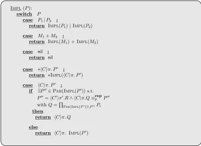
4.8 Definition of function Impl. . . 53

4.9 Axioms and rules to generate nameless tree representations of processes. . 57

4.10 Axioms and rules to generate nameless tree representations of conditions. . 58

4.11 Definition of function Box. . . 65

4.12 Pseudocode of the algorithm that verifies if two complexes are isomorphic. 68 4.13 Reduction semantics of BlenX. . . 70

4.14 Function Map. . . 72

5.1 Reduction semantics of Bcore. . . 83

5.2 Labelled transition semantics of Bcore. . . 86

5.3 Terminology and notation for action labels. . . 87

5.4 Reduction semantics of Bp_core. . . 103

5.5 Encoding of RAMs with Bp_core. . . 104

5.6 Reduction semantics of Be_core. . . 109

5.7 Encoding of RAMs with Be_core. . . 111

6.1 sBlenX syntax. . . 118

6.2 Reduction semantics of sBlenX. . . 120

6.3 Counting functions. . . 122

(12)

6.7 Immediate apparent probability and stochastic apparent rate. . . 149

6.8 Pseudo-code of the stochastic simulation slgorithm. . . 153

7.1 Different programs implementing enzyme catalysis . . . 159

7.2 Definition of identifiers, numbers and rates. . . 161

7.3 Declaration file BNF grammar. . . 162

7.4 Sorts file BNF grammar. . . 163

7.5 Program file BNF grammar. . . 164

7.6 Program file BNF grammar. . . 166

7.7 Definition of complexes . . . 167

7.8 Events file BNF grammar. . . 169

7.9 Definition of templates. . . 171

8.1 Complete code of the detailed MAPK cascade model (part 1). . . 186

8.2 Complete code of the detailed MAPK cascade model (part 2). . . 187

9.1 Generic EvolutionAlgorithm_{. . . 200}

(13)

List of Figures

2.1 Single substrate catalysed reaction. . . 12

2.2 Competitive inhibition. . . 14

2.3 Ordered sequential bisubstrate enzymatic reaction. . . 15

2.4 MAPK cascade. . . 16

3.1 Example of BlenX system. . . 31

3.2 Example of BlenX system dynamics. . . 34

4.1 Example of a complex. . . 42

4.2 Example of process tree representation. . . 55

4.3 Example of an event substituting a subpart of a complex. . . 72

6.1 Visual representation of a machine complex. . . 127

6.2 Visual representation of the binding of two machine complexes. . . 137

6.3 Visual representation of the unbinding of two machine complexes. . . 140

6.4 The data structures used by the simulation environment. . . 154

7.1 The logical strucure of BWB. . . 158

7.2 Simulation results of the enzyme catalysis programs. . . 160

7.3 Complex generated by the BlenX program. . . 168

8.1 Visual representation of three different state machine implementations. . . 177

8.2 Schematic representation of proteins sending and receiving signals. . . 178

8.3 Simulation results of the MAPK cascade simplified model. . . 181

8.4 Simulation results of the MAPK cascade detailed model. . . 188

8.5 Simulation results of the MAPK cascade detailed model with functions. . . 189

8.6 Example of compartimetalized space. . . 192

9.1 Different kinds of mutations. . . 203

9.2 Introducing a new domain. . . 205

(14)

9.6 Changes in fitness during a typical evolutionary simulation. . . 210

(15)

An answer is always the stretch of road that’s behind you. Only a question can point the way forward.

(16)

(17)

Chapter 1

Introduction

1.1

The context

Biology is the science of life and embraces many different disciplines and areas. One of these ismolecular biology, which aims at studying biology on a molecular level. Molecular biology deals with the formation, structure, and function of macromolecules essential to life (e.g., DNA, RNA and proteins) and hence overlaps with other areas of biology and chemistry, particularly genetics and biochemistry.

In the last thirty years, the constant advances in technologies and experimental tech-niques in molecular biology led to a massive increase in the data available to scientists. The application ofinformatics to store, manage and analyse this enormous amount of data results in what we call today bioinformatics. This first convergence between computing and biology conducted scientists to a deeper comprehension of the basic mechanisms gov-erning living organisms, leading to unthinkable achievements like the Human Genome Project that sanctioned the beginning of the post-genomic era.

(18)

a shift in the notion of what to look for in biology. While the understanding of genes and proteins continues to be important, the focus is on understanding the system’s structure and dynamics. Although subverting the traditional reductionist approach, this system-level perspective is not against it but throws the basis for a new paradigm that in the last years has been identified with systems biology. An explicit and precise definition of systems biology is difficult to give [57, 56, 110, 82, 52], or even still impossible, but we can capture its main principles and goals in the words of Kirschner [56]:

“I would simply say that systems biology is the study of the behaviour of complex biological organization and processes in terms of the molecular con-stituents. It is built on molecular biology in its special concern for information transfer, on physiology for its special concern with adaptive states of the cell and organism, on developmental biology for the importance of defining a succession of physiological states in that process, and on evolutionary biology and ecology for the appreciation that all aspects of the organism are products of selection, a selection we rarely understand on a molecular level. Systems biology attempts all of this through quantitative measurement, modelling, reconstruction, and theory.”

It is clear how systems biology is strongly inter-disciplinary and calls for the integration and convergence of many different sciences and disciplines. Its domain indeed spreads from several branches of biology to more distant disciplines, such as physics, mathematics, statistics and informatics. The main role of these latter distant disciplines is to devise adequate formal tools and concepts to describe and model efficiently biological systems, analyse their properties, and reproduce and predict their behaviour through computer-based simulations (e.g., [105, 66, 68, 70]), with the ultimate and challenging goal of delineating the basis for a foundation theory of systems biology.

Systems biology gave hence the opportunity to propel a further step into the con-vergence between informatics and biology already started years ago with bioinformatics, resulting in a moment of incredible scientific ferment where various computational ap-proaches have been proposed and equipped with supporting software tools (e.g., [96, 79, 40, 46, 49]). A computational model differs from a traditional mathematical one, be-cause it is executable and not just simply solvable [37]. Execution means that we can predict/describe the flow of control between species and reactions (e.g., not only the time, but also the causality relation among the events that constitute the history of the dynamics of the model).

(19)

CHAPTER 1. INTRODUCTION 1.2. THE PROBLEM

of application. This approach stresses the importance of concurrency and interaction be-tween molecules as the main tools that drive the execution of biological processes and is at the basis of emergent schools of thought like [92, 62]. Furthermore, it gave the opportunity to reuse several theoretical results and analysis techniques developed for concurrent and distributed systems into the realm of biological system, with the primary goal of bringing new insights on their functioning.

One of the first examples of application of these concepts can be found in [96], where a framework for modelling biological processes is developed around the π-calculus [73]. The π-calculus is probably the most famous representative of the process calculi family, invented to specify and study the behaviour of concurrent software systems through an hierarchy of formal specifications written in the same calculus more and more concrete till the implementation on a specific architecture [71, 50]. The peculiarity of describing a system at different levels of abstraction using the same calculus and the automatic gen-eration of intermediate states by the semantics rather than the need of specifying all of them since the beginning, make process calculi particularly suitable to model biological systems. Process calculi are provided also with stochastic variants, primarily developed as tools for analysing the performances of concurrent systems [91, 48]. Models constructed with these stochastic calculi are usually Continuous Time Markov Chains (CTMC), the same kind of stochastic processes used to directly simulate systems of biochemical re-actions under certain physical considerations [43]. This further analogy allowed to use stochastic simulation by means of Gillespie’s algorithm [42] also in the context of pro-cess calculi, denoting them definitely as a powerful abstraction for the representation of biological systems.

During the last years a number of process calculi have been developed for applications in systems biology (e.g., [10, 97, 26, 90, 94, 18]). On top of these process calculi several languages have been defined and frameworks for analysis and stochastic simulation have been implemented (e.g., [85, 16, 76, 1]). Some of these new bio-inspired process calculi differ from classical process calculi because they are devised from the beginning for biology and aim at overcoming some expressivity limitations by developing new conceptual tools. Motivated by the intention to take some significant step in this direction we started three years ago by exploring a new design space for process calculi with the aim to capture in an intuitive and simple way the fundamental mechanisms of biological modelling.

1.2

The problem

(20)

try to interpret, they mainly make models”.

A model is a partial representation of reality and its main aim is to show which are the necessary and sufficient characteristics of a system that allow to understand it. In [82], Noble says that the power of a model lies in identifying what is essential, whereas a complete representation would live us just as wise, or as ignorant, as before. Being the process calculi approach strictly related with the modelling activity, one the first question we have to ask ourselves when developing a new modelling language is: What do we expect from our language?

The initial aim of this thesis work was to design a language, based on the process calculi paradigm, for modelling and study signalling networks. The importance of being able to represent in an effective way the relevant mechanistic details of signal transduction systems is stressed also in [57] where Kitano states that “The most feasible application of systems biology research is to create a detailed model of cell regulation, focused on particular signal-transduction cascades and molecules to provide system-level insights into mechanism-based drug discovery”.

The main problem we have to deal with when we model signalling networks is the complexity of protein-protein interactions, i.e., the enormous number of possible post-translational covalent modifications of proteins and the formation of protein complexes. This problem is also called combinatorial explosion problem. Combinatorial explosion usually arises because: proteins sometimes exist in different species with common func-tionalities; proteins can present multiple conformational states (e.g., different combina-tions in sites phosphorylation) and still present the same functionalities; proteins can be part of different complexes and still present the same functionalities. In general, the number of reactions of systems presenting these characteristics grows exponentially with the number of protein species, protein domains and binding capabilities.

1.3

The contribution

(21)

CHAPTER 1. INTRODUCTION 1.3. THE CONTRIBUTION

accommodate possible distinct instances of the same macro-behaviour.

Recognizing that Beta-binders improves the abstract representation of biological in-teractions and considering this improvement fundamentally important for a realistic and effective representation of signalling pathways, we selected it as a basis for our work. Al-though maintaining the basic principles characterizing the soul of Beta-binders, the result of this work deviates substantially from it, hence justifying a different name for our new language, theBlenX language. BlenX inherits from Beta-binders the basic abstraction of biological entity (a process encapsulated into a box with interaction capabilities) and the notion of communication by compatibility. However, many new features are introduced. InBlenXwe introduce the notion ofevent, a reformulation of the join and split operations of Beta-binders. Moreover, we introducecomplexes. A complex is a combination of two or more proteins and molecules attached together along compatible surfaces. In BlenX

complexes are represented as graphs with boxes as nodes. Although similar to [26, 13], our interpretation of complexes is substantially different in the way complexes can be formed and modified. By extending the notion of compatibility, indeed, we enable also at the level of complexes generation the kind of non-determinism already characterizing the communication approach instantiated by Beta-binders.

The coarse-grained modelling level allowed by BlenX is also characterized by the pres-ence of a general mechanism for encoding high-level operations as sequpres-ences of low-level ones. The language is indeed enriched with priorities [19], a scheduling scheme that per-mits to compose sequences of low-level operations atomically. Priorities are essential to implement scenarios in which for example we want to describe atomically sequences of modifications happening on a whole complex.

It is clear how an interesting question is whether and how those modifications and new features affect the ability of BlenX to act as a computational device. Some first insights to this question are given in this thesis. We show indeed that for a core subset of the language termination is decidable. Moreover, we prove that by adding either priorities or events to this core language, we obtain Turing equivalent languages.

(22)

All the theoretical framework presented in this thesis is accompanied with the imple-mentation of a framework for validation and simulation purposes: The Beta Workbench (BWB). It is a collection of tools built on top of BlenX to model and simulate biological systems.

Having in our hand this framework for thein-silico experimentation we first investigate the modelling of signalling pathways, proposing general design patterns for the definition of them. Then, we propose a framework for simulating the evolution of protein-protein interaction networks where evolution proceeds through selection acting on the variance generated by random mutation events, and individuals replicate in proportion to their performance, referred to as fitness. Finally, we investigate the modelling of self-assembly, providing general design patterns for modelling non-trivial structures like filaments, trees and symmetric rings.

It is important to underline that the BlenX language is in continuous evolution and several extensions are currently subject of other parallel works. Here we present only the subset concerning my thesis work, the kernel part of BlenX, representing its heart.

1.4

Structure of the thesis

• Chapter 1 is this introduction;

• Chapter 2 gives basic preliminaries about biological systems, introduces process calculi and presents an overview of the main process calculi applied or developed for systems biology;

• Chapter 3 presents informally the BlenX language, providing an overview of its main features;

• Chapter 4 gives a formal presentation of the BlenX language and its operational semantics, and explores some theoretical properties regarding structural congruence and its decidability and complexity;

• Chapter 5 shows that for a core subset of the language termination is decidable. Moreover, it shows that by adding either global priorities or events to this core language, we obtain Turing equivalent languages;

• Chapter 6describes sBlenX, the stochastic extension ofBlenX. Moreover, it presents a stochastic abstract machine for sBlenX that, using results presented in Chapter 4, compresses the system state space;

(23)

CHAPTER 1. INTRODUCTION 1.5. RELATED PUBLICATIONS

• Chapter 8 investigates the modelling of signalling networks, providing models and design patterns (of increasing complexity) of the well know MAPK cascade signalling network;

• Chapter 9 describes a framework that allows the study of signalling networks evo-lution. A case study based on the MAPK cascade is presented.

• Chapter 10 investigates the modelling of self-assembly inBlenX, providing models and design patterns for the formation of non-trivial structures like filaments, trees and symmetric rings;

• Chapter 11 concludes and summarises the thesis.

1.5

Related publications

Book Chapters

L. Dematt´e, R. Larcher, A. Palmisano, C. Priami, A. Romanel. Programming Biology in BlenX_. _{In Systems Biology for Signaling Networks, Springer, 2010.}

L. Dematt´e, C. Priami, A. Romanel. The BlenX _{Language: A Tutorial}_. _{In SFM}

2008, LNCS 5016:313-365, Springer, 2008.

International journals

R. Larcher, C. Priami, A. Romanel. Modelling self-assembly in BlenX_. _Transactions

on Computational Systems Biology XII, LNBI 5945:163-198, Springer, 2010.

A. Romanel and C. Priami. On the Computational Power of BlenX_. _Theoretical

Computer Science 411(2):542-565, Elsevier, 2010.

L. Dematt´e, C. Priami, A. Romanel, O. Soyer. Evolving BlenX programs to simulate the evolution of biological networks. Theoretical Computer Science 408(1):83-96, 2008.

L. Dematt´e, C. Priami, A. Romanel. The Beta Workbench: a computational tool to study the dynamics of biological systems. Briefings in Bioinformatics 9(5):437-449, 2008.

(24)

Congruence for Beta-binders. Theoretical Computer Science 404(1-2):156-169, 2008. L. Dematt´e, C. Priami, A. Romanel. Modelling and simulation of biological pro-cesses in BlenX_. _{SIGMETRICS Performance Evaluation Review} _{35:32-39, 2008.}

International conferences and workshops

L. Dematt´e, C. Priami, A. Romanel, O. Soyer. A Formal and Integrated Framework to Simulate Evolution of Biological Pathways. In Proceedings of Computational Methods in Systems Biology (CMSB), Springer LNCS, 4695:106-120, 2007.

L. Dematt´e, C. Priami, A. Romanel. BetaWB: modelling and simulating biolog-ical processes. In Proceedings of Summer Computer Simulation Conference (SCSC), 777-784, 2007.

(25)

Chapter 2

Preliminaries

2.1

Biological systems

A cell is a microscopic structure containing nuclear and cytoplasmic material enclosed by a semipermeable membrane and, in plants, a cell wall. It is meant to be the basic structural unit of all organisms.

From a topological perspective, a cell can be seen as an architecture of physical brane bounded locations (i.e., compartments whose boundary are determined by mem-branes). Each compartment is a container of substances and the role it plays in regulating cell life depends on the substances that it contains. The content of compartments changes over time as a result of cell regulation. Consequently, substances continuously migrate from one location of the cell to another in response to internal and/or external stimuli.

An eukaryotic cell is made up of a plasma membrane that surrounds the internal sub-compartments, the organelles. The interior, or lumen, of each organelle is enclosed by one or more membranes and contains a unique set of proteins that characterizes the functions of the organelle together with the membrane-bound proteins. The largest organelle is the nucleus. The part outside the nucleus is called cytoplasm and it contains all the other organelles. The aqueous part of the cytoplasm is called cytosol and it contains a large number and variety of substances. These substances continuously produces a chemical activity that allows a cell to grow, multiply, and do its daily tasks.

The main categories of cell substances are listed in the following.

(26)

gene expression and reaction catalysis. The two main cellular processes involving DNA are replication and transcription. Replication is the process of making a complete copy of the DNA sequence and occurs whenever the cell divides. Transcriptions concerns the decodification of the information that is stored in the DNA sequence: DNA is transcribed into RNA while RNA is translated into proteins.

Proteins: they are essential parts of organisms and participate in almost every process within cells. They perform several different tasks, like reaction catalysis and regulation, transmission of signals, gene expression and regulation, membrane transport. Proteins are polymers of amino acids, called polypeptides. The sequence of amino acids is usually referred to as the protein’s primary structure and determines the protein’s three dimen-sional structure and shape, which is the key of its functioning. This structure depends on how the primary sequence folds around itself. Although the process of folding is still poorly understood, several studies revealed some local regularities in the folding pattern, called protein’s secondary structure. The secondary structure gives rise to elements called structural motifs (or domains) that allow the proteins to interact with other molecules. Besides local foldings, the overall three dimensional structure of a protein is called ter-tiary structure. When proteins complex with other proteins or molecules, the obtained structure is referred to as the quaternary structure. The way in which proteins function is extremely interesting. When they interact or combine with other proteins or molecules, they maintain their overall structure (their identity) but change their shape. The dif-ferent three dimensional shapes that proteins can assume are also called conformational states. For example, there are enzymes with active and inactive states; when active, these enzymes can bind to substrates and catalyse the corresponding reaction. The conforma-tional states and the binding capabilities of a protein define its behaviour and function.

Metabolites: a metabolite is an intermediate product of the metabolism. Metabolites can be fuels and signalling molecules, cellular building blocks, nucleotides, carbohydrates, lipids, hormones, vitamins, and various other molecules concerned with the vast range of cellular tasks. Usually, metabolites can perform very specific tasks and their structure and chemical properties are relatively simple if compared, for example, to proteins. We can think as if they have single identities and states. Indeed, if a metabolite reacts it becomes a different metabolite with a different identity and function.

2.1.1 Biochemical reactions

(27)

CHAPTER 2. PRELIMINARIES 2.1. BIOLOGICAL SYSTEMS

An example of reaction is:

2A+B →3C

MoleculesAandBarereactants, whileCis theproduct. When in a system this reaction happens, two moleculesAand a moleculeB will vanish, and three moleculesCwill appear. Values 2 and 3 are known as stoichiometries, and they are usually natural numbers. A molecule can be both consumed and produced in a single reaction. In particular, if a chemical species occurs on both the left and the right hand side, it is referred to as modifier. A reaction that can happen in both directions is known as reversible. Reversible reactions are quit common in biology. They are written explicitly adding a reverse arrow for the backward reaction:

2A+B ⇋₃_C

This notation is simply a shorthand for the two separate reaction processes taking place.

Chemical kinetics is concerned with the time-evolution of a reaction system specified by a set of coupled chemical reactions. In particular, it is concerned with the system behaviour away from equilibrium. Although the reaction equations capture the key in-teractions between substances, on their own they are not enough to determine the full system dynamics. The rates at which each of the reactions occurs, together with the initial concentration of the reacting molecules, are the missing information. The rate of a reaction is a measure of how the concentration of the involved substances changes with time. To better understand the crucial concept relating to the dependency between the rate and the concentration, let us consider one single stage reaction in which one molecule

A reacts with a moleculeB, giving one molecule of C.

A+B →C (2.1)

According to the collision theory, C is produced with a rate that is proportional to the hits frequency of A and B. Let us imagine to have a certain number of molecules

(28)

molecule. In our case we hence have:

rate = d[C]

dt =k[A][B]

where k is the basal rate and [A], [B] and [C] denote the concentration of molecules A,

B and C, respectively. In general, the rate is proportional to the concentration of the reactants involved raised to the power of their stoichiometry. For example, given the homogeneous1 _reaction:

nA+mB→P (2.2)

the corresponding relation between the rate and the concentration is:

rate= dP

dt =k[A]

n_[_B_]m _(2.3)

and the global order of the reaction corresponds to the sum of n and m.

2.1.2 Enzymatic catalysis

Enzymes play the important role of catalysing those biochemical reactions that make life possible. Basically, enzymes bind to one or more ligands, called substrates, and convert them into one or more chemically modified products. A simple enzymatic reaction is considered in Fig 2.1. This mechanism is also called single substrate catalysed reaction. The enzymeE and the substrateS encounter to form the enzyme-substrate intermediate ES. This reaction can be reversed, but the formation of ES is favoured when many substrates molecules are available. When S is bound, E sends a signal enabling the modification of the substrate S into product P. Finally, the product P is released, and the enzyme E regenerated.

P

E S

ES _EP

E

Figure 2.1: Single substrate catalysed reaction.

(29)

CHAPTER 2. PRELIMINARIES 2.1. BIOLOGICAL SYSTEMS

More concisely we can write this reaction as:

E+S −↽r⇀−1 r2

ES r3

−→EP r4

−→E+P

Note that only the first reaction is considered reversible. Indeed, many enzymatically catalysed reactions are irreversible, meaning that under normal conditions the backward reaction can be neglected.

Enzymatic catalysis is usually described by the Michelis-Menten kinetics. In this setting the single substrate catalysed reaction is represented using the formulation:

E+S −↽r⇀−1 r2

ES r3

−→E+P

that abstracts from the presence of the intermediateEP. The Michaelis-Menten equation describes the relationship between the rate of substrate conversion by an enzyme to the concentration of the substrate:

r= Vmax×[S]

Km+ [S] where,

Km= r2+r3

r1

and Vmax =k3×[E]t

In this equation,ris the rate of conversion,Vmaxis the maximum rate of conversion, [S] is the substrate concentration, andKm is the Michaelis constant. The Michaelis constant is equivalent to the substrate concentration at which the rate of conversion is half ofVmax.

Km approximates the affinity of enzyme for the substrate. A small Km indicates high affinity, and a substrate with a smaller Km will approach Vmax more quickly. Very high [S] values are required to approach Vmax, which is reached only when [S] is high enough to saturate the enzyme. While the derivation is not shown in this discussion, Vmax is equivalent to the product of the catalyst rate constant (k3) and the (total) concentration

of the enzyme.

Inhibitors are molecules that decrease the speed of enzymatic reactions. When an inhibitor binds to an enzyme it can prevent a substrate from entering the active domain of the enzyme or directly block the catalytic activity of the enzyme. The action of an inhibitor can be either reversible or irreversible. A particular type of reversible inhibition, namedcompetitive inhibition, is sketched in Fig. 2.2. In this mechanism the substrate S

(30)

inhibi-P

E S

ES _EP

E

I

EI

Figure 2.2: Competitive inhibition.

tion is:

E+S −↽r⇀−1 r2

ES r3

−→E+P

E+I −↽r⇀−5 r6

EI

The derivation of the Michaelis-Menten equation is the same as for the uninhibited mechanism except for an additional term in the expression that accounts for the total enzyme concentration and for the new intermediate EI. The derived equation is:

r= Vmax×[S]

Km+ [S] +Km× r6 r5

×[I]

More complicated forms of enzymatic reactions are given by multi-substrate catalysed reactions, where more substrates are involved in the process. A large group of these reac-tions are the bisubstrate reactions, which have two substrates. For bisubstrate reactions three basic reaction mechanisms have been discerned: the ordered sequential mechanism, the random sequential mechanism and the ping pong mechanism. As an example, in the first mechanism (see Fig. 2.3) the enzyme first binds both substrates and then proceeds to the actual catalytic reaction step; the substrates can only bind in a given order.

2.1.3 Signalling networks

(31)

CHAPTER 2. PRELIMINARIES 2.1. BIOLOGICAL SYSTEMS

P1

S1

E

ES1

S2 ES1S2 EP1P2

EP2

P2

E

Figure 2.3: Ordered sequential bisubstrate enzymatic reaction.

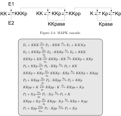
second messengers. Biological signal transduction allows a cell or organism to sense its environment and react accordingly. Typically, a signalling network has one (or more) in-puts, represented by any environmental stimulus, and one (or more) outin-puts, represented by an active protein. The types of signals that are transmitted are numerous: synaptic signals transmitted by neurons, signals indicating the presence of harmful substances, signals indicating to single cells that another cell is ready to mate, and signals transmit-ted through hormones that convey a whole range of cellular instructions. An example of signalling network is the MAPK cascade.

The MAPK cascade: The mitogen-activated protein kinase cascade (MAPK cascade) is a series of three protein kinases2 _{which is responsible for the cell response to some}

growth factors. In [51], a model of the MAPK cascade was presented and analysed using Ordinary Differential Equations (ODEs); the cascade was shown to perform the function of an ultra-sensitive switch and the response curves were shown to be steeply sigmoidal. Fig. 2.4 presents schematically MAPK cascade as described in [51]. KKK denotes MAP-KKK, KK denotesMAPKK and K denotes MAPK. The signal E1 transforms KKK to KKKp, which in turn transformsKK toKKp toKKpp, which in turn transformsK toKp to Kpp. In particular, when an input E1 is added, the output of Kpp increases rapidly. The transformations in the reverse direction are the result of the signal E2, the KKpase and theKpase. In particular, by removing the signalE1, the output level of Kpp reverts back to zero. The formal model in [51] is built using 30 single reactions (see Tab. 2.1). The set of reactions is used to derive a system of 25 mathematical equations (18 ODEs plus 7 conservation equations).

2_{a kinase is a type of enzyme that transfers phosphate groups from high-energy donor molecules, such as}_ATP_,

(32)

Figure 2.4: MAPK cascade.

E1+KKK a1

−⇀ ↽−

d1

E1 :KKK k1

−→E1+KKKp

E2+KKKp a2

−⇀ ↽−

d2

E2:KKKp k2

−→E2+KKK

KKKp+KK−↽a⇀−3

d3

KKKp:KK−→k3 KKKp+KKp P2+KKp

a4

−⇀ ↽−

d4

P2 :KKp−→k4 P2+KK

KKKp+KKp−↽a⇀5−

d5

KKKp:KKp−→k5 KKKp+KKpp P2+KKpp

a6

−⇀ ↽−

d6

P2 :KKpp k6

−→P2+KKp

KKpp+K −↽a⇀7−

d7

KKpp:K k7

−→KKpp+Kp P1+Kp

a8

−⇀ ↽−

d8

P1:Kp k8

−→P1+K

KKpp+Kp−_↽a⇀₋9

d9

KKpp:Kp k9

−→KKp+Kpp P1+Kpp

a10

−−⇀ ↽−−

d10

P1 :Kpp−−→k10 P1+Kp

Table 2.1: MAPK cascade reaction set.

2.2

Stochastic simulation

Given a set of coupled chemical reactions describing a biological system, one of the most immediate and natural analyses that can be performed on it is a simulation. The term simulation is generally used to indicate the calculation of the system’s dynamics over time, given an initial specific system configuration; for biological systems the initial configura-tion corresponds usually to the initial concentraconfigura-tion of molecules.

Biological systems can be simulated in different ways using different algorithms de-pending on the assumptions made about the underlying kinetics. Once the kinetics have been specified, these systems can be used directly to construct full dynamic simulations of the system behaviour on a computer.

(33)

ther-CHAPTER 2. PRELIMINARIES 2.2. STOCHASTIC SIMULATION

modynamic limit (i.e., system’s volume and molecules quantities approach infinite, while keeping their ratio constant). Given these assumptions, ODEs models aredeterministic: given an initial configuration, their dynamics is univocally determined. However, the ther-modynamic limit cannot be always assumed, because in many systems some molecules quantity can be very low. In these cases, microscopic random effects arise, making the system naturally stochastic. Chemical stochastic systems are usually represented by a chemical master equation (CME) that describes the time evolution of the probability distribution of the discrete molecule quantities (expressed by natural numbers). This evolution is a Continuous Time Markov Chain (CTMC), of which any possible realisa-tions can be generated through Monte Carlo sampling methods. The most famous of these methods for coupled chemical reactions is the SSA algorithm of Gillespie [42, 43].

2.2.1 Gillespie algorithm

Gillespie designed an efficient way to simulate a trajectory of a set of coupled chemical reactions. The algorithm he proposed is exactly consistent with the underlying princi-ples behind the CME [42, 43]; it simulates a jump Markov process and is based on the assumption that two events take place at the same time with zero probability.

In [43] a generic system of coupled chemical reactions is described as a vector S =

(S1,· · · , Sn), representing a well-stirred mixture of n ≥ 1 interacting molecular species,

confined in constant volume Ω and containingM ≥1 reaction channels (chemical reactions described by stoichiometric equations) R = (R1,· · · , Rm). The dynamics of a system is

specified by a vector of random variables X(t) = (X1(t),· · · , Xn(t)), where Xi(t) is the

population of the species Si present in the system at time t. Given X(t) = x, for each reaction channel Rj, there exists a function aj(x), called propensity function, defined as the probability that a reactionRj occurs in the next infinitesimal time interval [t, t+dτ). The functionaj(x) is defined asaj(x) =cj×hj(x) and its result is denoted withpropensity value. Constant cj, for the corresponding channel Rj, represents the specific probability rate constant and consists of a base rate determined empirically and dependent on the specific type of reaction plus some environmental conditions. Function hj(x), instead, returns the number of all the possible distinct reactions that can occur between molecules on channel Rj, when the system is in state x. Vectors S, R, X(t) together with the functionaj(x), for each j ∈ {1,· · ·, m}, completely specify the system at time t.

(34)

First Reaction Method (FRM)

At each step a random putative reaction time is calculated for each reaction and the one with the shortest time is chosen and executed.

1. Set the initial number of molecules for each species in S

2. Set t←0

3. Calculate the propensity value ai for each i∈ {1,· · · , m}

4. For each i∈ {1,· · · , m} generate a putative time τi in accordance with an exponential distribution of parameter ai

5. Let τµ and µ be the fastest time τj and the corresponding reaction channel Rj

6. Update the number of molecules to reflect the execution of µ

7. Set t←t+τµ

8. Return to step 3

Direct Method (DM)

Two separate calculations are considered: the selection of the reaction and the evaluation of the time. The dynamics of the system is described by the following density function: (1) P(j | x) = aj(x)/Pm_i₌₁ai(x), that is the probability that the next reaction is on channel j; (2)P(τ | x) = (P_im₌₁ai(x))e−τ(Pm

i=1ai(x)). The pseudo-code of the algorithm is

defined as follows:

1. Set the initial number of molecules for each species in S

2. Set t←0

3. Calculate the propensity value ai for each i∈ {1,· · · , m}

4. Choose reaction channel µ in accordance with distribution (1) 5. Choose time τ in accordance with distribution (2)

6. Update the number of molecules to reflect the execution of µ

7. Set t←t+τ

8. Return to step 3

Next Reaction Method (NRM)

(35)

CHAPTER 2. PRELIMINARIES 2.3. PROCESS CALCULI IN SYSTEMS BIOLOGY

• Reaction dependency graph: By using a reaction dependency graph, during the sim-ulation the algorithm needs only to update those propensities which it knows could have changed. Reaction dependency in biological pathways is typically much less than m and hence the reaction dependency graph issparse;

• Indexed priority queue: Reaction times are arranged in a indexed priority queue [21]. The root holds the reaction with the faster time and the reactions further from the root always have longer times than those closer. Reactions at the same height are not ordered. The fastest reaction is selected in O(1). When the reaction with the root time is executed, its propensity and those of the set of dependent reactions changes, along with the corresponding times in the priority queue. Since it is not necessary to maintain a horizontal ordering, the authors provide an algorithm which applies pairwise exchanges of reaction times at adjacent heights in the tree to maintain the tree’s invariant property. This has complexity proportional to the number of reaction times that change multiplied by the height of the tree. Since it has already been assumed that the average reaction dependency of the system is sparse, the overall complexity of selecting a reaction becomes O(log m).

Another minor advantage is obtained by considering absolute times. By considering reaction times relative to t0, thus absolute time, the NRM is able to re-use the putative

times of reactions whose propensities have been changed by the firing of the selected reaction. In this way the NRM needs only to generate one random number per simulation step, hence reducing the computational cost related with random numbers generation.

2.3

Process calculi in systems biology

Several approaches have been developed and used to model and study complex interac-tion mechanisms in biological systems, mainly based on mathematical modelling, which generally takes the form of a system of ordinary differential equations (ODEs) and for which ODE solvers with various interfaces are available.

(36)

to solve mathematical formulations of problems. Various computational approaches have been proposed and equipped with supporting software tools (e.g., boolean networks [55], Petri nets [46], Bayesian networks [40], graphical gaussian models [80], process calculi [96], rule-based modelling [49]).

We consider in this thesis the process calculi paradigm, that we believe can pro-vide an interesting abstraction to an executable philosophy of computational modelling. Process calculi indeed have the ability of handling concurrency, execution causality, non-determinism, stochastic behaviour and cooperation/competition for resources that are usual features of computational approaches.

2.3.1 Overview of process calculi

Starting from the Calculus of Communicating Systems [71] (CCS), process calculi have been defined to provide us with formal specifications of concurrent systems, i.e., compu-tational entities executing their tasks in parallel and able to synchronise. The model of a system S is typically given as a term that defines the possible behaviours of the various components ofS. Calculi are equipped with syntax-driven rules, the so-called operational semantics [88]. These rules allow to infer the possible future of the system under analysis and can be automatically implemented. For instance, they can specify that a certain system P evolves into system Q, written P → Q. The basic entities of process calculi are names, an abstract representation of the interaction capabilities of processes. Names are used to build elementary computations, called actions and co-actions (complementary actions). In the most basic view, like e.g., in CCS, an action is seen as an input or an output over a channel. Input and output are complementary actions. The actual inter-pretation of complementarity varies from one calculus to the other. The relevant fact to be pointed out here is that complementary actions are those that parallel processes can perform together to synchronise their (otherwise) independent behaviours. A process is computational unit that evolves by performing actions (a, b, · · ·) and co-actions (e.g. a,

b, · · ·). The possible temporal order of the concurrent activities is specified by a limited

set of operators. Sequential ordering is rendered via the prefix operator written as an infix dot. For instance the term a.b.P denotes a process that may execute the activity a, then b, and then all the activities modelled by P. Two processes P and Q that run in parallel are represented by the infix parallel composition operator|as in P |Q. Processes

P and Qcan either evolve independently or synchronise over complementary actions. For instance, the operational semantics of a.P |a.Q allows to infer the transition:

(37)

CHAPTER 2. PRELIMINARIES 2.3. PROCESS CALCULI IN SYSTEMS BIOLOGY

Another operator is the choice operator, written +. The process P +Q can proceed either as the process P or the process Q, meaning that the two behaviours are mutually exclusive. For instance, the operational semantics of a.P | a.Q+a.R allows to infer the transitions:

a.P | (a.Q+a.R)→P |Q and a.P | (a.Q+a.R)→P | R

Another essential operator is the restriction. In basic calculi as CCS, this operator, written (νa), is meant to limit the visibility of actions. For instance, is not possible to infer a.P | (νa)a.Q → P | (νa)Q because a is a private resource of the right-hand process of the parallel composition and the left-hand process cannot interact on it. This fact guarantees, e.g., that the two processes R and S in (νa)(R | S) may interact over

a without any interference by the external world. In more sophisticated calculi, as the

π-calculus [73], the restriction operator ensures a relevant gain in expressiveness. As in CCS, the view about complementarity is limited to input and output over channels. Over CCS, however, theπ-calculus allows to send channel names in interactions. This permits the representation of mobile (i.e., dynamically changing) systems: receiving new names means acquiring new interaction capabilities.

Infinite behaviours are usually obtained in process calculi by using operators like repli-cation, denoted by !P, which allows one to create an unbounded number of parallel copies of a process P, all placed at the same level. Other mechanisms to generate infinite be-haviours arerecursion and iteration [77].

Above we recalled only the fundamental operators which are common to various pro-cess calculi [71, 73]. Each calculus then adopts some specific operators and has a specific view about which activities must be considered complementary. A common feature of process calculi is that their operational semantics allows to interpret process behaviours as a graph, called transition system. The nodes of the graph represent processes, and there is an arc between the two nodes P and Q if P can evolve to Q. For instance the immediate future of P =a.P1 | a.P2 | a.P3 is drawn as:

P →P1 |P2 | a.P3 and P →a.P1 | P2 | P3

The depicted transitions highlight that botha.P1 anda.P3can communicate witha.P2.

(38)

The behaviour of a complex system is expressed in terms of the meaning of its com-ponents. A model can be designed following a bottom-up approach: one defines the basic operations that a system can perform, then the whole behaviour is obtained by compo-sition of these basic building blocks. This property is called compositionality. Moreover, the mathematical rules defining the operational semantics of process calculi allow to au-tomatically generate the transition system of a given process by parsing the syntactic structure of the process itself. So, process calculi are specification languages that can be directly executed.

Process calculi are provided also with stochastic variants, primarily developed as tools for analysing the performances of concurrent systems [91, 48]. In these variants, process calculi are usually decorated with quantitative information representing the speed and probability of actions; these information are used to derive a CTMC.

2.3.2 Process calculi abstractions

The abstraction introduced by Regev and Shapiro in [98] (see Tab. 2.2), opened the realm of process calculi to the field of systems biology. A molecule is seen as a computation unit, a process, with interaction capabilities abstracted as channels names. Molecules interact/react through complementary capabilities as processes communicate on channels with the same name (action and co-action). The change of a state after a communication abstracts the dynamics of a molecule after a reaction.

Biology Process calculi

Molecule Process

Interaction capability Channel

Interaction Communication

Dynamics State change

Table 2.2: Process calculi abstraction for systems biology.

Stochastic extensions of process calculi, moreover, allows to describe the same kind of stochastic processes used to directly simulate systems of coupled chemical reactions. This analogy allowed to use stochastic simulation by means of SSA Gillespie’s algorithm also in the context of process calculi, denoting them definitely as a powerful abstraction for the representation of biological systems.

(39)

CHAPTER 2. PRELIMINARIES 2.3. PROCESS CALCULI IN SYSTEMS BIOLOGY

process calculi proposed in the last years. It is interesting to note that the various calculi are developed to study a particular aspect, i.e., they abstract a specific (or a set of) char-acteristic of a biological system. Indeed, an approach founded on language theory allows to fast develop specific calculi that are hypothesis driven.

Biochemical π-calculus[96]: it is the first process calculus used to represent biological systems. In biochemical π-calculus, complementary domains of interaction are repre-sented by channel names and co-names; molecular complexes and cellular compartments are rendered by the appropriate use of restrictions on channels; molecules interaction ca-pabilities are represented by communication. Moreover, since the calculus is stochastic, the behaviour of biological system can also be described and analysed quantitatively. Two simulators for the biochemical stochasticπ-calculus have been implemented: BioSPI [96] and SPiM [85]; this simulators implement the DM of Gillespie. Moreover, interesting ap-plications of biochemicalπ-calculus on real biological scenarios can be found in [67, 15, 61].

Performance Evaluation Process Algebra (PEPA) [48]: it is a formal language for describing CTMC. PEPA allows to quantitatively model and analyse large pathway systems. PEPA is supported by a large community and a lot of software tools for analy-sis and stochastic simulations are available. Moreover, in [17] the authors show how the combined use of PEPA and the probabilistic model checker PRISM [45] can be used to describe, simulate and analyse biochemical signalling pathways. Recently, an extension called Bio-PEPA [18] has been introduced. In this extension PEPA is modified to deal with some features of biological models, such as stoichiometry and the use of generic ki-netic laws. The language is provided with a complete set of tools for performing various kinds of analyses [16].

(40)

of BioAmbients models are presented.

Brane Calculi [10]: it is a calculus focused on biological membranes, which are not considered only as containers, but are active entities. A system is viewed as a set of nested membranes and a membrane as a set of actions. Brane Calculi primitives are in-spired by membrane properties; membranes can merge, split, shift or act as channels. In [27], an extension called Projective Brane Calculus is presented. The goal of the extension is to refine Brane Calculi with directed actions, which tell whether an action is looking inwards or outwards the membrane. This modification brings the calculus closer to bi-ological membranes. Recently, to improve the consistency with bibi-ological characteristics of membrane reactions, a new extension has been proposed in [28]. This extension uses a generalized formalism for action activation with a receptor-ligand type channel construc-tion that incorporates multiple associaconstruc-tion and a concept of affinity.

CCS-R [25]: it is a CCS-like process calculus which allows the management of reversibil-ity. Reversibility is embedded in the syntax of the calculus, which is equipped with memories that trace communications and backtrack them when needed. It is not clear whether the main features of CCS-R are relevant for modelling biological systems, because the fact that the system obtained after backtracking a reaction is the same as the initial one is still debated.

(41)

CHAPTER 2. PRELIMINARIES 2.3. PROCESS CALCULI IN SYSTEMS BIOLOGY

The π@ calculus [109]: it is an extension of the π-calculus, obtained by the addition of polyadic synchronisation and priorities. The expressiveness of the calculus is shown in [107] by providing encodings of bio-inspired formalisms like BioAmbients and Brane calculi. The language is provided with a stochastic variant (the Sπ@) that is shown to be able to model consistently several phenomena such as formation of molecular complexes, hierarchical subdivision of the system into compartments, inter-compartment reactions, dynamic reorganisation of compartment structure consistent with volume variation.

The continuous π-calculus [63]: it is process calculus for modelling behaviour and variation in molecular systems. Processes are parallel combinations of species, where species are very similar to π-calculus processes. Communication is through named chan-nels, but there is no distinction between names and co-names. Any name can in principle communicate with any other; an affinity matrix specifies whether any two names can communicate and at what rate. The calculus is provided with an operational semantics in terms of real vector spaces, that offers a fully modular and compositional method of generating a set of ordinary differential equations (ODEs). The calculus is specifically designed to study evolutionary properties of biological systems.

The attributed π-calculus [54]: it is an extension of the π-calculus with attributed processes and attribute dependent synchronization. The calculus is parametrized with a call-by-value λ-calculus, which defines possible values of attributes. The calculus is provided with a non-deterministic and a stochastic semantics, where stochastic rates may depend on attribute values.

Bigraphs [74]: they are conceived as a unifying framework for designing models of con-current and mobile systems. These reactive systems are construed as a set of rewriting rules together with an initial bigraph on which the rules operate. The main entities of bigraphs are nodes and named edges; nodes are arranged in a tree structure, they have prescribedarities telling how many edges must be incident to them, and edges can con-nect arbitrarily many nodes. In [60], a stochastic version of bigraphs is presented, along with some examples of their applicability in some biological domains.

(42)

individually. Only processes that are sufficiently close can communicate.

(43)

Part I

(44)

(45)

Chapter 3

Informal presentation

BlenXis a language thought to deal with the complexity of protein-protein interaction. It is inspired by Beta-binders and hence has a process calculi soul. Although maintaining the basic principles characterizing Beta-binders, BlenX deviates substantially from it, hence justifying a different name. BlenX inherits from Beta-binders the abstraction used to represent biological substances (processes encapsulated into boxes with interfaces) and the notion of communication based on compatibility. It is important to underline that one important difference betweenBlenX and Beta-binders is that BlenX omits the restriction operator in the description of processes. Its expressive power is recovered by using a set of constructs that fit better in the biological context. These new features are:

• complexes: boxes can bind (and unbind) through interfaces to form (and break down) graphs of boxes, called complexes. Bindings between interfaces are dedicated links that allow enclosed processes to communicate in an exclusive way. Binding and unbinding operations are obtained by extending the notion of compatibility of Beta-binders;

• priorities: they provide a mechanism to encode high-level operations as sequences of low-level ones. InBlenX, priorities are associated with actions and are represented by positive natural numbers where one assumes that greater is the number, greater the priority it represents. The priority protocol we implement is global, meaning that actions with higher priority prevents the execution of all the actions with lower priority.

(46)

the communication primitives;

• conditions: the execution of primitives can be prevented by conditions that check the state of the box interfaces. They allow to condition the internal behaviour of boxes depending on the actual configurations that box interfaces can assume.

The direct application of BlenX to biological modelling is accomplished by providing a stochastic variant of BlenX. In such an extension, the language is decorated with quan-titative information which are used to derive the speed and the probabilities associated with actions, as usual in the stochastic setting.

3.1

BlenX

on the road

BlenX represents a biological substance as a computational object, a box, composed by a set of interfaces and an internal process. Interfaces are associated with structures, that we call sorts, and are the places where a box can interact with other boxes; the internal process, instead, codifies for the mechanism that transforms an interaction into a box structure modification. In this setting, a protein can be represented as a box, its domains by interfaces, and protein conformational states can be described by internal processes.

We use the following graphical notation of boxes:

B is the box andP is its internal process that describes its behaviour. Intuitively,P is used to program proper replies to external signals caught by the interfaces (which are the small squares on the border of the box). Sorts ∆1, ∆2 and ∆3 discriminate among allowed

and disallowed interactions, mimicking the interaction mechanism based on compatibility described in [90]. The names x1, x2 and x3 are used by the process P to modify or to

interact through the associated sorts ∆1, ∆2 and ∆3, respectively. Process P is written

in a process calculi style; it has few primitives inspired by π-calculus, extended with primitives inspired by molecular biology [2].

(47)

CHAPTER 3. INFORMAL PRESENTATION 3.1. BLENXON THE ROAD B1 P1 C D E B3 P3 D E B2 P2 A D F B4 P4 E B2 P2 A D F B2 P2 A D F B2 P2 A D F B3 P3 D E B3 P3 D E B3 P3 D E B3 P3 D E B3 P3 D E B4 P4 E B4 P4 E B4 P4 E B4 P4 E B4 P4 E B1 P1 C D E B1 P1 C D E B1 P1 C D E B1 P1 C D E B1 P1 C D E B3 P3 D E B3 P3 D E B4 P4 E B2 P2 A D F B2 P2 A D F

Figure 3.1: Example of BlenX system.

chapter and we put here the language on the road by considering the single substrate catalysed reaction presented in Sec. 2.1.2. We will present three different implementations, giving hence an overview of all the main features of BlenX.

Using complexes

Enzyme and substrate can be modelled inBlenXby the parallel composition of two boxes

E and S, written E k S, representing the enzyme and the substrate, respectively:

The primitive x!sig, in the internal process of E, sends a signal sig through the interface (x,∆E). Symbol∗indicates the replication operator (typical operator of process

calculi that allows for the generation of infinite behaviours) and assures that the process sends a signal each time it is needed, i.e., each time the substrate and the enzyme interact. The primitivey?sig, in the internal process ofS, waits for a signal on the interface (y,∆S)

that enables the change of its sort in ∆P, by means of ch(y,∆P) action.

(48)

symmetric function α that, given a pair of sorts, returns a triple of values. For instance,

α(∆E,∆S) = (1,1,1) (3.1)

means that the sorts ∆E and ∆S, associated with the interfaces of the boxes E and S,

may bind, unbind and communicate, respectively; the three type of actions are enabled over a certain pair of sorts only if the corresponding values are greater than zero. The result of α(∆E,∆S) in (3.1) allows hence inferring the following reaction enabled in the

system E k S:

The two boxes bind over their interfaces with sorts ∆E and ∆S, respectively, creating a

link that only they can use. Following Fig. 2.1, the reaction that leads to the intermediate form enzyme-substrate can be reversed, namely the boxes E and S can unbind. This is represented by the following pictorial reaction:

Their unbind is allowed because the corresponding value in the result of α(∆E,∆S)

in (3.1) is greater than zero. However, instead of breaking up the binding, the enzyme-substrate complex can undergo certain modifications that lead to the release of the prod-uct. This is modelled in BlenX as a communication over the link created between the two interfaces through the binding, followed by a change in the sort of the interface (y,∆S).

In particular, the process ∗x!sig can send a signal sig through the interface (x,∆E); the

process y?sig.ch(y,∆P) can receive a signal from the interface (y,∆S) and subsequently

(49)

CHAPTER 3. INFORMAL PRESENTATION 3.1. BLENXON THE ROAD

Note that the internal process of the box E is not changed because the replication operator∗ allows to regenerate the outputx!sig each time it is consumed.

The internal processch(y,∆P) of the box S′ changes the sort of the interface (y,∆S)

from ∆S to ∆P, completing the transformation from substrate S to product P. This

transformation is described by the following reaction:

The processnilin the reaction products is the empty process. Note that more complex behaviour can be specified for the resulting productP.

Looking back to Fig. 2.1, the last step of enzymatic catalysis is the release of the product and the regeneration of the enzyme. The unbind of boxesE and P is guaranteed by assuming:

α(∆E,∆P) = (0,2,0) (3.2)

that prescribes that each time the types ∆E and ∆P are bound they have to unbind. The

zeros in the first and third positions mean that types ∆E and ∆P cannot bind and cannot

interact if they are bound. Theα result (3.2) allows inferring the following reaction:

(50)

Figure 3.2: Example of BlenX system dynamics. Normal arrows represent the dynamics as-sociated with single reactions, while dashed arrows represent the dynamics of more than one reaction.

biological world, where, e.g., internal modifications of the structure of a complex are in competition with some environmental solicitations that lead a complex to break. We will see in the next chapter how the operational semantics of BlenX allows for the automatic construction of such a transition system.

(51)

CHAPTER 3. INFORMAL PRESENTATION 3.1. BLENXON THE ROAD

putting it in parallel with the existing enzymes and substrates. If we assume this box to have an interface (x,∆I) and we update the α function definition by adding the relation α(∆E,∆I) = (1,1,0), then we can infer the following dynamics:

The inhibitor I can bind to the enzyme E, hence preventing the creation of the inter-mediate enzyme-substrate.

Using communication

In the previous example we have assumed that a communication between different boxes can happen only thorugh formed links. This is true only if the α specification of the corresponding interface sorts contains values for bind and unbind that are not both equal to zero. As we will see more in detail in the next chapter, if an α specification is equal to (0,0, n) with n >0, then binding and unbinding are not contemplated for the pair of sorts and the boxes exposing them can communicate without the need of first creating a link. To show this we consider a simplification of the enzyme activation example where an interaction between and enzyme and a substrate leads to the release of the product without the generation of intermediate complexes.

By specifying an affinity like the following:

α(∆E,∆S) = (0,0,1) (3.3)

we have that the initial system composed by an instance of an enzyme and a substrate can evolve as follows:

(52)

Using events

The primitives we described above work mainly with elementary reactions. In our setting, with elementary reactions we identify those reactions that do not abstract any intermedi-ate configuration with respect to a certain known biological mechanism. In the previous example, indeed, the language primitives allowed us to model the reactions and the inter-mediate configurations of enzyme activation in detail, by maintaining also the identity of the single biological components. However, it is generally difficult to describe biological systems only in terms of elementary reactions, because there are scenarios in which the underlying biological mechanisms are not known with enough detail. In these cases, the application of the primitives described above results difficult. Thus, to deal also with these scenarios we introduce events.

Events implement a class of rewriting rules that substitute sets of boxes with other sets of boxes. In order to better explain how events work, we consider again the previous enzyme catalysis example and model it only by using events. In this setting, we can model the enzyme, the substrate, the intermediate complexes and the product as different boxes:

The initial configuration of the system can be modelled by Ee k Se. The binding and the unbinding of the enzyme and the substrate can be modelled by two different events. The first one substitutes the configurationEe k Se withESe, meaning that a box representing the enzyme and a box representing the substrate are substituted with a box representing their complexation:

(53)

CHAPTER 3. INFORMAL PRESENTATION 3.1. BLENXON THE ROAD

Also events can be associated with priorities and here we assume all the considered events to have the same priority 1. Having generated a box ESe we can describe the transformation of the intermediate complex and the release of the product directly using an event that substitutes the box ESe with the parallel composition of boxes Pe k Es, abstracting also from the reaction that in the previous model was associated with an higher priority:

(54)

(55)

Chapter 4

Syntax and semantics

4.1

Syntax and notation

LetN be a countably infinite set of names (ranged over byx,y, n, x1,x′, · · ·) and letT

be a finite set ofsorts (ranged over by ∆, Γ, ∆′_{, ∆}

0, · · ·) such that T ∩ N =∅.

ABlenXsystem, written (B, E, ξ), is a triple made up of a bio-processB, a composition of eventsEand an environmentξ. We denote withSthe set of all possible systems (ranged over byS, S′_, _S

1,· · ·).

Tab.4.1 presents the complete syntax of the language. Hereafter, to simply the pre-sentation, we will overload function names and symbols when unambiguous.

Bio-processes are generated by the non-terminal symbol B and with B we denote the set of all possible bio-processes (ranged over by B, B′_, _B

1, · · ·). A bio-process can

be either empty ( Nil ), a box ( I[P ]n ) or the parallel composition of bio-processes

( B0 k B1 ). In the definition of box I[P]n, I represents its interaction capabilities, P

is its internal engine, and n is used as an identifier to address the box at hand. Given a bio-processB, the function Boxes(B) is used to extract the set of boxes composing B.

I is a non-empty string of interfaces of the form K(x, ∆)p_{, where} _K _{denotes the}

state of the interface, which can be either free ( ⊕ ) or bound ( ⊗ ), the name x is the subject of the interface, ∆ is a sort representing its structure, and p ∈ N is a