lsasim: an R package for simulating large-scale assessment data

lsasim: an R package for simulating

large‑scale assessment data

Tyler H. Matta

_{, Leslie Rutkowski}

_{, David Rutkowski}

_{and Yuan‑Ling Liaw}

Introduction

Large‑scale assessments in education

An important tool for monitoring educational systems around the world, interna-tional large-scale assessments (ILSAs) are cross-nainterna-tional, comparative studies of achievement. ILSAs are used to measure educational achievement in select content domains for representative samples of students enrolled in primary and secondary educational systems. The achievement tests that students take are intended to be an adequate representation of what students know and can do in the relevant content areas (e.g., math, science, and reading). And the results of these assessments are used to compare educational systems (usually, but not exclusively, countries) and to inform policy, practice, and educational research both nationally and internationally. In terms of numbers of participants, these studies have grown tremendously over the past few decades. Today, two-thirds of all countries with populations greater than 30,000 have participated in one or more international or regional large-scale assessments (Lock-heed et al. 2015). Among the most well-known ILSAs are the Trends in International Mathematics and Science Study (TIMSS) and the Programme for International Stu-dent Assessment (PISA). On a 4 year cycle, beginning in 1995, TIMSS measures math-ematics and science in a representative sample of fourth and eighth grade students. Starting in 2000 and every 3 years afterward, PISA assesses 15-year-olds enrolled in

Abstract

This article provides an overview of the R package lsasim, designed to facilitate the generation of data that mimics a large scale assessment context. The package features functions for simulating achievement data according to a number of common IRT models with known parameters. A clear advantage of lsasim over other simulation software is that the achievement data, in the form of item responses, can arise from multiple‑matrix sampled test designs. Furthermore, lsasim offers the possibility of simulating data that adhere to general properties found in the background question‑ naire (mostly ordinal, correlated variables that are also related to varying degrees with some latent trait). Although the background questionnaire data can be linked to the test responses, all aspects of lsasim can function independently, affording researchers a high degree of flexibility in terms of possible research questions and the part of an assessment that is of most interest.

Open Access

© The Author(s) 2018. This article is distributed under the terms of the Creative Commons Attribution 4.0 International License (http://creativecommons.org/licenses/by/4.0/), which permits unrestricted use, distribution, and reproduction in any medium, provided you give appropriate credit to the original author(s) and the source, provide a link to the Creative Commons license, and indicate if changes were made.

SOFTWARE ARTICLE

school in math, science, and reading. Besides the subject assessment (e.g. math, sci-ence, and reading tests), these studies also solicit information from students, their teachers, principals, and their parents regarding beliefs, attitudes, experiences, and the context of schooling. With over half a million students from 70 educational sys-tems taking part, PISA is now the largest such study (OECD 2017). New versions of PISA, such as PISA for Development, targeting developing economies, and PISA for schools, focused on providing participating schools with internationally comparable results, will only increase these numbers and bring international assessments to new contexts and audiences. The quantitative nature, scale, and scope of these and related modern educational surveys necessitates a fairly sophisticated approach to the survey design, sampling, analysis, and reporting. We elaborate subsequently.

The first such study, the Pilot Twelve-Country Study (Foshay et al. 1962) was rev-olutionary at the time—before email, the Internet, and fast, desktop computers. By modern standards of educational and psychological measurement AERA, APA, and NCME (2014), however, the study was primitive, using classical test theory methods to uncover data of relatively low quality on a single test form. Beginning with the 1995 cycle of TIMSS, international assessments adopted an item response theory-based approach to scaling and a sophisticated booklet design, referred to as multiple matrix sampling (MMS) (Shoemaker 1973). Essentially, MMS is a method that divides test items into non-overlapping blocks that are then assembled into booklets according to, typically, a variant of a balanced incomplete block design (Gonzalez and Rutkowski

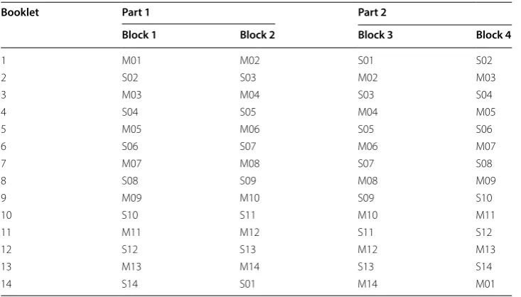
2010; Rutkowski et  al. 2014). The result is, in the case of most international large-scale assessments (ILSAs), 10 or more hours of testing content delivered in two-hour booklets (Martin et al. 2016; OECD 2017). A concrete example, located in Table 1, is the 2011 Trends in International Mathematics and Science Study (TIMSS) design that distributed 429 total mathematics and science items across 14 non-overlapping math-ematics blocks and 14 non-overlapping science blocks.

Table 1 2011 TIMSS booklet design

Booklet Part 1 Part 2

Block 1 Block 2 Block 3 Block 4

1 M01 M02 S01 S02

2 S02 S03 M02 M03

3 M03 M04 S03 S04

4 S04 S05 M04 M05

5 M05 M06 S05 S06

6 S06 S07 M06 M07

7 M07 M08 S07 S08

8 S08 S09 M08 M09

9 M09 M10 S09 S10

10 S10 S11 M10 M11

11 M11 M12 S11 S12

12 S12 S13 M12 M13

13 M13 M14 S13 S14

Only a fraction of the students in the sample take any one item, and any selected student takes only a fraction of the total available items. As a result, the actual distribution of stu-dent proficiency cannot be approximated by its empirical estimate (Mislevy et al. 1992b). Further, traditional methods of estimating individual achievement introduce an unaccepta-ble level of uncertainty and the possibility of serious aggregate-level bias (Little and Rubin

1983; Mislevy et al. 1992a). As one means for overcoming the methodological challenges associated with multiple-matrix sampling, large-scale assessment programs adopted a pop-ulation or latent regression modeling approach that uses marginal estimation techniques to generate population- and subpopulation-level achievement estimates (Mislevy 1991; Mis-levy et al. 1992a, b)

More specifically, using information from background questionnaires, other demo-graphic variables of interest and responses to the cognitive portion of the test, student achievement is estimated via a latent regression model, where achievement (θ ) is treated as a latent or unobserved variable for all examinees. Essentially, the limited achievement test responses, complete student background questionnaires responses, and select demo-graphic information are used in conjunction with a measurement model-based extension of Rubin’s (1987) multiple imputation approach to generate a proficiency distribution for the population (or sub-population) of interest (Beaton and Johnson 1992; Mislevy et al. 1992a,

b; von Davier et al. 2006). A short, slightly more technical description follows.

As in multiple imputation methods, an imputation model (called a “conditioning model”) is used to derive posterior distributions of student achievement. This model uses all avail-able student data (cognitive as well as background information) to generate a conditional proficiency distribution from which to draw a number of plausible values (usually five) for each student on each latent trait (e.g. mathematics, science, and associated sub-domains).

Because θ is a latent, unobserved variable for every examinee, it is reasonable to treat it

as a missing value and to approximate statistics involving θ by its expectation. That is, for any statistic, t, _tˆ_{(X, Y)=E[t(θ ), Y|X, Y] =}

t(θ, Y)p(θ|X, Y)dθ where X is a matrix of achievement item responses for all examinees and Y is the matrix of responses of all exami-nees to the set of administered background questions. Because closed-form solutions are typically not available, random draws from the conditional distributions are drawn for each sampled examinee j (Mislevy et al. 1992b). In line with missing data practices (Rubin 1976,

1987), values for each examinee are drawn multiple times. These are typically referred to as plausible values in LSA terminology or multiple imputations in missing data literature. Using Bayes’ theorem and the IRT assumption of conditional independence,

where P(xj|θ ) is the likelihood function for θ and p(θ|yj) is the distribution of θ for a given vector of response variables. Usually, it is assumed that θ is normally distributed according to the following model

where ǫj∼N(0,) and Ŵ and have to be estimated.

(1) p(θ|xj, yj)∝P(xj|θ, yj)p(θ|yj)=P(xj|θ )p(θ|yj),

The role of simulations in large‑scale assessment research and development

In the past 20 years, national and international assessments have expanded significantly in terms of the number of national- or system-level participants, platforms (comput-erized in addition to paper and pencil), content domains (e.g., collaborative problem solving), and the degree to which participating countries differ in economic, cultural, linguistic, geographic, and other terms. To that end, two areas of research in large-scale assessment are evaluating the performance of currently used methods given the chang-ing nature of LSAs and developchang-ing new methods. In both cases, areas of emphasis can conceivably include test design, administration, data collection, sampling, or other rel-evant areas. As study administrators are naturally cautious about implementing new designs and methods without evidence of their merit and worth, a viable option for test-ing new methods is through simulation. Further, ustest-ing empirical data to examine the performance of current and new methods is limited by the fact that we can never know the true, underlying population values of item- or person-parameters. Simulation is a low-cost powerful means for conducting methodological research in the area of large-scale assessment. Examples include Adams et al. (2013), Rutkowski and Zhou (2015).

Traditionally, the mandate of large-scale assessments surrounds measuring and reporting achievement across populations of interest. As such, large-scale assessment developers prioritize achievement measures, in terms of framework development, psy-chometric quality, analysis, and reporting (OECD 2014; Martin et al. 2016). Neverthe-less, background questionnaires serve to contextualize educational achievement and provide opportunities to understand correlates of learning. To that end, the background questionnaire and achievement measures have distinct frameworks, and different teams work to develop and innovate in each respective area. This (in some cases arbitrary) distinction between the achievement test and background questionnaires frequently leads researchers to regard each component separately for many methodological inves-tigations. Therefore, lsasim (Matta et al. 2017) simulates data in a way that treats back-ground questionnaire responses as separate from but related to the achievement test.

Software for generating large‑scale assessment data

The goal of lsasim is to provide a set of functions that enable users to design and modify test designs that are commonly utilized in large-scale educational surveys. Such goals are similar to the goals of catR (Magis and Raiche 2012) for generating item response patterns from computer adaptive tests and mstR (Magis et al. 2017) for generating item response patterns from multi-stage tests. The difference, however, is that multi-matrix sampling designs utilized in large-scale assessments are not (yet) adaptive, and can thus, depend on other packages to estimate item parameters and achievement estimates.

In addition to the inability to generate item responses under a multi-matrix sampling designs, none of the IRT packages reviewed provide a means for generating responses to “background questionnaires,” data that are commonly used in the estimation of achievement. To include responses to background variables, one would need to develop functions on their own, or utilized an alternative package to generate mixed normal, bivariate, and ordinal data such as GenOrd (Barbiero and Ferrari 2015).

With lsasim designed to generate item responses, it has no functionality to estimate item parameters or achievement estimates. For this, users should turn to existing pack-ages, for example, TAM, as is demonstrated later in this article. The data output from lsasim is formatted to be used with TAM or mirt without any further data manipula-tion. Furthermore, the ibd package (Mandal 2018) can be used in tandem with lsasim to generate balanced incomplete designs.

Simulation methodology

Generating correlated questionnaire data

Let X= {X1,X2,. . .,Xp,. . .,XP} be a set of continuous random variables and

W = {W1,W2,. . .,Wq,. . .,WQ} be a set of ordinal (possibly dichotomous) ran-dom variables. For any Wq , let there be 1,. . .,kq,. . .,Kq ordered response catego-ries where p(Wq=kq)=πq,k such that

1≤k≤Kπq,k =1 . Furthermore, let R , be a (P+Q)×(P+Q) possibly heterogeneous correlation matrix which includes (a) Pear-son product-moment correlations for ρ(Xp,Xp′) ; (b) polychoric correlations for any ρ(Wq,Wq′) ; and (c) polyserial correlation for any ρ(X_p,W_q).

Often in the development of psychological tests, items are designed with the assump-tion that ordinal item responses map to a continuous latent trait. Thus, we can specify an underlying continuous variable, W_q⋆ , for any ordinal variable, Wq . The relationship

between Wq and Wq⋆ is

where α_q,k is the kth threshold for Wq⋆ , delineating responses k−1 and k on the scale of W⋆

q.

To simulate correlated mixed-type data, we need only a (P+Q)×(P+Q) data-generating correlation matrix, R and the Kq marginal probabilities πq corresponding to

each ordinal variable Wq . First, generate N replicates from P+Q independent standard

normal random variables Z= {Z(X1),. . .,Z(XP),. . .,Z(W1⋆),. . .,Z(WQ⋆)} , such that an N×(P+Q) data matrix, Z , is obtained. Second, let L be the lower triangle matrix of the Cholesky factorization of R where R=LL′ . We can transform Z to {X, W⋆} using L such that {X, W⋆} =ZL . Finally, we transform the latent variables W⋆ to W by coarsening based on Eq. 3.

(3) Wq=                   

1 if , − ∞ <W⋆

q ≤αq,1 2 if , αq,1 <W_q⋆ ≤αq,2 ..

.

k if , α_q,k−1 <W_q⋆ ≤αq,k ..

.

Generating IRT‑based data

In order to generate data from many models in the IRT-family, we specify an overly general model accompanied by explicit constraints, given the generating informa-tion. The general model combines the three-parameter model for dichotomous item responses and the generalized partial credit model for ordered responses,

where k is the response to item i by respondent j, θj is the respondent’s true score, and Ki

is the maximum score on item i. Furthermore, bi is the average difficulty for item i, diu is

the threshold parameter between scores u and u−1 for item i, ai is the item’s

discrimi-nation parameter, ci is the item’s pseudo-guessing parameter, and D is a scaling constant

for the item.

Because the partial credit model does not, generally, include a guessing parame-ter, we place constraints on parts of the model given the known parameters. Namely, when multiple thresholds are specified for a given item, u>1 , the pseudo-guessing parameter is constrained to zero, c=0 , resulting in the generalized partial credit

model. Further constraining a=1 results in the partial credit model. When only one threshold is specified, Eq. 4 reduces to

From here, constraining c=0 results in the two-parameter item response model and

constraining c=0,a=1 results in the Rasch model.

The lsasim package

The lsasim package contains a set of functions that facilitate the generation of large-scale assessment data. The package can be divided into two interrelated sets of func-tions: one set for generating background questionnaire data and another set for generating the cognitive data. This section provides a description of each function within the package and demonstrates how they can be used. To start, we set a seed for replicability purposes and load the lsasim package and the polycor package (Fox

2016), both available on CRAN.

(4) p(uij =k|θj)=ci+(1−ci)

expk

u=1Dai(θj−bi+diu)

Ki

v=1exp v

u=1Dai(θj−bi+diu)

(5) p(yij=k|θj)=ci+(1−ci)

exp

Dai(θj−bi)

1+exp

Dai(θj−bi)

Background questionnaire data

The main function for generating background questionnaire data is aptly named

questionnaire_gen. The function facilitates the generation of correlate continu-ous, binary, and ordinal data by specifying the cumulative proportions for each back-ground item and a correlation matrix.

The n_obs argument specifies the number of observations (examinees) to generate. The argument cat_prop takes a list of vectors, each of which contain the cumulative proportions for a given background item. The length of the list, that is, the number of vectors within the list, indicates the number of background items to be generated. Each vector in the list should end with 1 such that the length of each vector specifies the num-ber of response categories for that background item. For continuous items, the vector should contain one element, 1.

The code above provides an example of cumulative proportions for two background items. The first background variable has one category, indicating a continuous response. The second background item has four response categories with marginal population proportions of 0.23, 0.31, 0.27, and 0.19, respectively.

In the above example, we specify a polyserial correlation of .7 between the discrete background item and the continuous item. Notice that the size of ex_cor is equal to the length of the ex_prop as the size and order of cor_matrix corresponds to

cat_prop.

Using ex_prop and ex_cor, we simulate one dataset with 1000 observations. By default, continuous variables are generated from standard normals, N_{(0, 1) .}

Notice the continuous variable q1 is a numeric variable and the discrete variable q2

is a factor with four levels. A third variable, subject, is the unique identifier for each observation. With our simulated data set, we see the first two moments of q1 and the marginal proportions for q2 are both well-recovered.

Additionally, the polyserial correlation is also well-recovered using the hetcor

function from the polycor package.

It is important to note that converting the factor variables to numeric and estimat-ing a Pearson correlation will not recover the generatestimat-ing correlation matrix.

The questionnaire_gen function includes three optional arguments, c_mean,

and c_sd takes a vector of standard deviations. The lengths of c_mean and c_sd are equal to the number of continuous items to be generated. Specification of c_mean

and/or c_sd results in a continuous variables i to be distributed N(c_mean[i],

c_sd[i]). Finally, theta is a logical argument where theta = TRUE results in the first continuous background item to be named “theta” in the resulting data frame. This optional argument is only for convenience when generating both background questionnaire data and cognitive data.

Notice in the example above, the continuous variable is now named theta and has a mean and standard deviation close to that specified by c_mean and c_sd.

The proportion_gen function generates a list of random cumulative propor-tions using two arguments. The first argument cat_options takes a vector whose entries specify the types of items to be generated. In the code below, cat_options

= c(1, 2, 3) specifies continuous, two-category, and three-category item types to be generated. The second argument, n_cat_options is a vector of equal length to cat_options, which specifies the number of each item type to be generated. Below, n_cat_options = c(3, 2, 1) indicates that there will be three con-tinuous items, two two-category items, and one three-category item generated (six items in all).

Cognitive data

The cognitive assessments for LSAs are much more involved than the background ques-tionnaire. As mentioned above, the cognitive assessments use an IRT measurement model administered using a multi-matrix sampling scheme. The package lsasim has been designed to provide researchers with extensive flexibility in varying these design features while providing valid default solutions as an option. There are five functions that make up the cognitive data generation, which we organize here under three cat-egories (a) item parameter generation: item_gen; (b) test assembly and administration:

block_design, booklet_design, and booklet_sample; and (c) item response generation: response_gen.

Item parameter generation

Although researchers may wish to use pre-determined item parameters, the item_gen

function enables the flexible generation of item parameters from item response models.

The arguments n_1pl, n_2pl, and n_3pl specify how many one-, two-, and three-parameter items will be included in the item pool. For this example, we will generate five two-parameter items and ten three-parameter items. The argument

c_bounds specify the bounds of the uniform distributions used to generate the b,

a, and c parameters, respectively. Note that a_bounds are only applied to the two- and three-parameter items and c_bounds are applied to three-parameter items only.

The above example shows the item information for the 15 items in item_pool. All 15 items have a bi parameter, which is the average difficulty for the item. The five two-parameter items were specified as generalized partial credit items with two thresholds. Thus, item 1 though item 5 have two d parameters, d1 and d2 such that bi+dik is the kth threshold for item i. All 15 items have a discrimination parameter, ai , while only item 6 through item 15 have a c parameter (pseudo-guessing). The

last two variables in item_pool, k and p, are indicators to identify the number of thresholds and whether the item is from a 1PL, 2PL, or 3PL model, respectively.

Test assembly and administration

non-overlapping blocks of items that can be assembled into test booklets. Two func-tions, block_design and booklet_design, facilitate the assembly of the test booklets while one function, booklet_sample facilitates the administration of the booklets to subjects. The test assembly process was split into two functions to provide users ample flexibility of how tests are constructed.

Block design

The first step in the test assembly is to determine the number of blocks and the assign-ment of items to those blocks. The function block_design facilitates this process with two required arguments and one optional argument. The n_blocks argument specifies the number of blocks while the item_parameters argument takes a data frame of item parameters. The default allocation of items to blocks is a spiraling design. For 1, 2,. . .,H item blocks, the first item is assigned to block 1, item 2 is assigned to the

block 2, and item H is assigned to block H. The process is continued such that item H+1 is assigned to block 1, item H+2 is assigned to block 2 and item H+H is assigned to

block H until all items are assigned to a block.

The function block_design produces a list that contains two elements. The first ele-ment, block_assignment, is a matrix that that identifies which items from the item pool correspond to which block.

The column names of block_assignment begin with b to indicate block while the rows begin with i to indicate item. For block b1, the first item, i1, is the first item from

item_pool, the second item, i2, is the fifth item from item_pool, the third item, i3, is the ninth item from item_pool, and the fourth item, i4, is the 13th item from item_ pool. Because the 15 items do not evenly distribute across 4 blocks, the fourth block only contains three items. To avoid dealing with ragged matrices, all shorter blocks are filled with zeros.

The second element in block_ex is a table of descriptive statistics for each block.

For user-specified block construction, we can specify an indicator matrix where the number of columns equals the number of blocks and the number of rows equals the number of items in the item pool.

The 1s indicate which items belong to which blocks. Given the example above, we will assign items 1 through 4 to block 1, items 5 though 8 to block 2, items 9 through 12 to block 3 and items 13 though 15 to block 4. Below, block_ex2 demonstrates how the matrix is used with the item_block_matrix argument and the items in

Booklet design

book_ex uses the default item-block assembly of block_ex. In the above output, book

B1 contains the items from block 1 and block 2, booklet B2 contains the items from block 2 and block 3, booklet B3 contains the items from block 3 and block 4, and book B4 con-tains the items from block 1 and block 4. Notice that the first two test booklets contain eight items while the last two books contain seven items. This is because block 4 only has three items whereas blocks 1, 2, and 3 have four times. Like block_design, booklet_ design avoids ragged matrices by filling shorter booklets with zeros.

Users can also explicitly specify the booklet assembly design using the optional argument

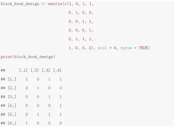
book_design. By specifying a booklet design matrix, users can control which item blocks go to which booklets. The book_design argument takes an indicator matrix where the columns indicate the item blocks and the rows indicate the booklets. In the code below, we create a matrix, block_book_design, that will create six test booklets. Booklet 1 (row 1) will include items from blocks 1, 3 and 4 while booklet 6 (row 6) will include items from block 1 only.

Table 2 Default booklet design Booklet Item blocks

b1 b2 b3 b4 . . . bH₋2 bH₋1 bH

B1 1 1 0 0 ... 0 0 0

B2 0 1 1 0 ... 0 0 0

. . . . . . . . . . . . . . . ._. . . . . . . . . . .

BN−1 0 0 0 0 ... 0 1 1

Notice how booklets B1 and B5, contain 11 items each while booklets B2 and B6 con-tain four items each.

Booklet administration

The final component of the test assembly and administration is the administration of test booklets to examinees. The function booklet_sample facilitates the distribu-tion of test booklets to examinees. The two required arguments are n_subj, the num-ber of examinees, and book_item_design, the output from booklet_design. The default sampling scheme makes all books equally likely but the optional argument

book_prob takes a vector of probabilities to make some books more or less likely to be administered. The logical argument resample will resample booklets until the differ-ence in booklets sampled is less than e or iter attempts. The resampling functionality may be useful when n_subj is small and only one dataset is being generated.

The result is a data frame with three columns: subject, book, and item. The data frame is organized in a long (univariate) format where there is one row for each sub-ject-item combination. The long format is required for generating item responses with the response_gen function. As can be seen in the output above, subject 1 has been administered booklet 2 while subject 2 has been administered booklet 4.

Item response generation

Recall that the item_gen function enables the user to specify different combinations of item response models for a given item pool. The response_gen function will gen-erate item responses for all models given four required arguments and five optional arguments.

Both arguments subject and item take length-N vectors that provide the subject by item information where N =

1:Jnj where nj is the number of items in the test for

the total number of items in the item pool. The optional arguments a_par and c_par

also take I-length vectors for the corresponding item parameters, while d_par takes an

I-length list where each element in the list is an (Ki−1)-length vector containing the thresholds for each item. The argument item_no is used only when a subset of items are used from a given item pool. Finally, the argument ogive allows the user to omit the scaling constant for a logistic ogive (default) or to include a normal ogive, ogive =

“Normal”.

The result of response_gen is a wide (multivariate) data frame where there is one row per examinee and each item is a column with the final variable indicating the sub-ject ID. Because not every examinee sees every item, items not administered are consid-ered missing.

Combining cognitive and background questionnaire data

Note that this section provided a general overview of the lsasim package. Interested readers can turn to the lsasim wiki for further documentation and testing results. In particular, one can find vignettes that further illustrate item parameter generation, test assembly, and test adminstration.

Generating data from PISA 2012

In this section, we demonstrate how existing background information, item parameters, and booklet designs can be used to generate data. The lsasim package includes prepared data from the 2012 administration of Programme for International Student Assessment.

PISA 2012 background questionnaire

The lsasim package includes the cumulative probabilities and heterogeneous correlation matrix for 18 background questionnaire items and a single mathematics plausible value. The 18 items comprise three scales, perseverance, openness to problem solving, and atti-tudes toward school. The cumulative proportions and correlation matrix were estimated using Switzerland student questionnaire data available from the PISA 2012 data base. It is important to note, however, that this background information is included for demon-stration purposes only and is not suitable for valid inferences.

With these two pieces of information, we can generate background questionnaire responses and mathematics scores for 1000 test takers. Notice that the variable names in

PISA 2012 mathematics assessment

The measurement model used in the 2012 administration of PISA was a partial credit model (OECD 2014). The technical manual provides the item parameters for all 109 mathematics items (OECD 2014,  pp. 406–409), which are stored in pisa2012_ math_item. Notice that each item has an item name, an item number, a b param-eter, and, for those partial credit items, two d parameters.

The PISA technical manual also provides information regarding the allocation of the 109 items to ten item blocks (OECD 2014,  pp. 406–409). pisa2012_math_block

Because only the indicator component of pisa2012_math_block is needed, we subset it and coerce it to a matrix. The PISA 2012 item parameters and correspond-ing block design matrix are used to create the block assignment matrix. Printcorrespond-ing the

block_descriptives provides a quick check of the block lengths and average difficulties.

The booklet design information for the PISA mathematics assessment was also trans-lated to a book design matrix, pisa2012_math_booklet (OECD 2014, p. 31). Like the block design, the book design is also stored as a data frame object to include a vari-able for booklet IDs. Note that this matrix was designed to construct the 13 standard

The 13 standard books can now be administered to the 1000 test takers.

Because we have excluded the easy booklets, not all 109 items will be used to gen-erate responses. Because the response_gen function matches item informa-tion based on a unique item number, we must subset the item bank to exclude those items in pisa2012_math_item that were not administered in the standard test books. To accomplish this, first obtain a sorted vector of unique items adminis-tered to the test takers, subitems. This vector can be used to subset the item bank,

pisa2012_math_item.

The resulting object, pisa_items, contains item information for the 84 adminis-tered items. Because we are using a subset of items whose item numbers are not sequen-tial, we use the optional argument item_no when using the response_gen function. The variables of the resulting data frame are renamed to the PISA 2012 items names.

Test design simulation study

We now conduct a simple simulation to demonstrate that the default test generating functions operate as intended.

One hundred one-parameter items were generated using the item_gen function. Those items were distributed across five item blocks, which were assembled into 5 booklets. Each booklet contained 40 items. Both the item block assembly and booklet assembly use the default spiraling design described above.

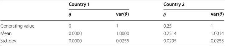
A true score, θ , was generated for 10,000 test takers in two countries (5000 test tak-ers in each country). For the first country, θ ∼N_{(0, 1) while for the second country,}

θ ∼N_{(0.25, 1)} . The five booklets were distributed evenly across the two countries and

country-specific means and variances were estimated using TAM (Robitzsch et  al.

Discussion

unique set of requirements on the test design and psychometric modeling. Although innovations in ILSAs can come from the re-analysis of past assessments, those data are fundamentally constricted to a particular design and by extant data. Due to the scope of ILSAs, pilot testing is highly restricted, leaving simulation studies as the primary means for understanding issues and possible solutions within the ILSA arena. The inten-tion for lsasim was to develop a minimal number of functions to facilitate the genera-tion of data that mimics the large scale assessment context to the extent possible. To that end, lsasim offers the possibility of simulating data that adhere to general proper-ties found in the background questionnaire (mostly ordinal, correlated variables that are also related to varying degrees with some latent trait). The package also features func-tions for simulating achievement data according to a number of common IRT models with known parameters. A clear advantage of lsasim over other simulation software is that the achievement data, in the form of item responses, can arise from multiple-matrix sampled test designs. Although the background questionnaire data can be linked to the test responses, all aspects of lsasim can function independently, affording researchers a high degree of flexibility in terms of possible research questions and the part of an assessment that is of most interest. Built in default functionality also allows researchers to opt for randomly chosen population parameters. Alternatively, users can specify their own test design specifications and population parameters, offering the possibility of full control over the research design and data generation process.

By way of introduction, the paper described and briefly illustrated the eight functions that make up the package. Because researchers will in many circumstances use informa-tion from previous assessments for simulainforma-tion purposes, the paper went on to demon-strate how LSA data can be generated from parameter estimates and design features of PISA 2012. Finally, a small simulation showed that using the default test assembly func-tions recovered known population proficiency parameters for two groups. Although we demonstrated the soundness of the package’s default settings, we expect users to rely on those default settings only for aspects of a given simulation design that are considered to be nuisances. For example, a study designed to examine the efficiency of various item block designs could rely on the default background questionnaire functions without loss of generality. Alternatively, a researcher interested in studying background questionnaire invariance across heterogeneousness populations might utilize many of the default test assembly functions. Otherwise, we generally assume that users will bring a set of known or plausible population parameters that will provide the basis for further investigations. We believe that lsasim can be a useful tool for operational test developers and basic and applied measurement researchers. As national and international assessments branch Table 3 Simulation results, means and standard deviations of country-specific parameters based on 100 replications

Country 1 Country 2

¯

θ var(θ) θ¯ var(θ)

Generating value 0 1 0.25 1

Mean 0.0000 1.0000 0.2514 1.0014

into new platforms and populations, it is important that researchers with a solid back-ground in measurement and large-scale test design have a ready means for evaluating the performance of new and existing methods. Finally, as a reminder, the default PISA parameters that are included with lsasim are not intended to be used to infer anything about the 2012 PISA administration. Rather, they provide an illustrative example of a test design and associated parameters that approximates an operational setting.

Authors’ contributions

The concept for lsasim was fostered by LR and DR. THM carried out the development of lsasim. YL led the test‑ ing of lsasim. THM, LR and DR contributed to the writing of the manuscript. All authors read and approved the final manuscript.

Author details

1 _{Pearson, San Antonio, TX, USA.} 2 _{Centre for Educational Measurement, University of Oslo, Oslo, Norway.} 3 _{Indiana Univer‑} sity, Bloomington, IN, USA.

Acknowledgements

The authors acknowledge Dr. Eugenio Gonzalez for his feedback during development as well as the Norwegian Research Council for supporting this research.

Competing interests

None of the authors have any competing interests that would be interpreted as influencing the research and ethical standards were followed in the conduct of lsasim and the writing of this manuscript.

Availability of data and materials

The package lsasim, including data used in this manuscript, can be found on Comprehensive R Archive Network, CRAN.

Funding

This manuscript was partially funded by the Norwegian Research Council, FINNUT program, Grant 255246.

Publisher’s Note

Springer Nature remains neutral with regard to jurisdictional claims in published maps and institutional affiliations.

Received: 9 May 2018 Accepted: 10 November 2018

References

Adams, R. J., Lietz, P., & Berezner, A. (2013). On the use of rotated context questionnaires in conjunction with multilevel item response models. Large-scale Assessments in Education, 1(1), 5.

American Educational Research Association, American Psychological Association, & National Council on Measurement in Education. (2014). Standards for educational and psychological testing 2014. AERA.

Barbiero, A., & Ferrari, P. A. (2015). GenOrd: Simulation of discrete random variables with given correlation matrix and marginal distributions [Computer software manual]. Retrieved from https ://CRAN.R‑proje ct.org/packa ge=GenOr d (R packa ge versi on 1.4.0)

Beaton, A. E., & Johnson, E. G. (1992). Overview of the scaling methodology used in the national assessment. Journal of Educational Measurement, 29(2), 163–175.

Chalmers, R. P. (2012). mirt: A multidimensional item response theory package for the R environment. Journal of Statistical Software, 48(6), 1–29. Retrieved from http://www.jstat soft.org/v48/i06/

Foshay, A. W., Thorndike, R., Hotyat, F., Pidgeon, D., & Walker, D. (1962). Educational achievement of thirteen-year-olds in twelve countries (Tech. Rep.). Hamburg: UNESCO Institute for Education. Retrieved from http://unesd oc.unesc o.org/ image s/0013/00131 4/13143 7eo.pdf

Fox, J. (2016). polycor: Polychoric and polyserial correlations [Computer software manual]. Retrieved from https ://CRAN.R‑ proje ct.org/packa ge=polyc or (R packa ge versi on 0.7‑9)

Gonzalez, E., & Rutkowski, L. (2010). Principles of matrix booklet designs and parameter recovery in large‑scale assess‑ ments. IERI Monograph Series, 3, 125–156.

Little, R. J. A., & Rubin, D. B. (1983). On jointly estimating parameters and missing data by maximizing the complete‑data likelihood. The American Statistician, 37(3), 218–220.

Lockheed, M., Prokic‑Breuer, T., & Shadrova, A. (2015). The experience of middle-income countries participating in PISA 2000–2015. Washington, DC: World Bank Publications. https ://doi.org/10.1787/97892 64246 195‑en.

Magis, D., & Raiche, G. (2012). Random generation of response patterns under computerized adaptive testing with the R package catR. Journal of Statistical Software, 48(8), 1–31. https ://doi.org/10.18637 /jss.v048.i08.

Magis, D., Yan, D., & von Davier, A. (2017). mstR: Procedures to generate patterns under multistage testing [Computer software manual]. Retrieved from https ://CRAN.R‑proje ct.org/packa ge=mstR (R packa ge versi on 1.0)

Martin, M. O., Mullis, I. V. S., & Hooper, M. (Eds.). (2016). Methods and procedures in TIMSS 2015. Boston: TIMSS & PIRLS Inter‑ national Study Center, Boston College. Retrieved from http://timss andpi rls.bc.edu/publi catio ns/timss /2015‑metho ds.html

Matta, T., Rutkowski, L., Rutkowski, D., & Liaw, Y. (2017). lsasim: Simulate large scale assessment data [Computer software manual]. Retrieved from https ://CRAN.R‑proje ct.org/packa ge=lsasi m (R packa ge versi on 1.0.0)

Mislevy, R. J. (1991). Randomization‑based inference about latent variables from complex samples. Psychometrika, 56(2), 177–196.

Mislevy, R. J., Beaton, A. E., Kaplan, B., & Sheehan, K. M. (1992a). Estimating population characteristics from sparse matrix samples of item responses. Journal of Educational Measurement, 29(2), 133–161.

Mislevy, R. J., Johnson, E. G., & Muraki, E. (1992b). Scaling procedures in NAEP. Journal of Educational and Behavioral Statis-tics, 17(2), 131–154.

OECD. (2014). PISA 2012 technical report (Tech. Rep.). Paris: OECD Publishing. Retrieved from https ://www.oecd.org/pisa/ pisap roduc ts/PISA‑2012‑techn ical‑repor t‑final .pdf

OECD. (2017). PISA 2015 technical report (draft). Paris: OECD Publishing.

R Core Team. (2017). R: A language and environment for statistical computing [Computer software manual]. Vienna: R Core Team. Retrieved from https ://www.R‑proje ct.org/

Robitzsch, A., Kiefer, T., & Wu, M. (2017). TAM: Test analysis modules [Computer software manual]. Retrieved from https :// CRAN.R‑proje ct.org/packa ge=TAM (R packa ge versi on 2.0‑37)

Rubin, D. B. (1976). Inference and missing data. Biometrika, 63(3), 581–592. Rubin, D. B. (1987). Multiple imputation for nonresponse in surveys. Hoboken, NJ: Wiley.

Rutkowski, L., von Davier, M., Gonzalez, E., & Zhou, Y. (2014). Assessment design for international large‑scale assessment. In L. Rutkowski, M. von Davier, & D. Rutkowski (Eds.), Handbook of international large-scale assessment: Background, technical issues, and methods of data analysis. Boca Raton: Chapman & Hall/CRC Press.

Rutkowski, L., & Zhou, Y. (2015). The impact of missing and error‑prone auxiliary information on sparse‑matrix sub‑popu‑ lation parameter estimates. Methodology, 11(3), 89–99.

Shoemaker, D. M. (1973). Principles and procedures of multiple matrix sampling. Oxford: Ballinger.