Scalable Computing: Practice and Experience
Volume 18, Number 3, pp. 229–241. http://www.scpe.org
ISSN 1895-1767 c
⃝2017 SCPE
DESIGN AND ANALYSIS OF MODIFIED SIQRS MODEL FOR PERFORMANCE STUDY OF WIRELESS SENSOR NETWORK
RUDRA PRATAP OJHA, GOUTAM SANYAL ∗, PRAMOD KUMAR SRIVASTAVA†, AND KAVITA SHARMA ‡
Abstract. The dynamics of worm propagation in the Wireless Sensor Networks (WSNs) is one of the fundamental challenge due to critical operational constraints. In this paper we propose a modified Susceptible-Infectious-Quarantined-Recovered-Susceptible (SIQRS) model based on epidemic theory. The proposed model demonstrate the effect of quarantined state on worms propagation in WSNs. This model incorporates communication radius, area of communication and the associated node density. The spreading dynamics of worms defined with the help of Basic Reproduction Number (R0) and ifR0is less than or equal to one the worm-free
equilibrium is globally asymptotically stable, and if R0 is greater than one the worm will persists in the system. This model
formulated by differential equations and explain the process of worm propagation in WSNs. We also study the effect of different parameters on the performance of system. Finally, the control mechanism and performance of the proposed model is validated through extensive simulation results.
Key words: Epidemic model, Basic reproduction number, Stability, Wireless Sensor Network, Communication radius, Node density
AMS subject classifications. 68M10, 90B18
1. Introduction. Data communication is one of the primary requirements of modern society. There are different ways of data communication,it may be wired and wireless. The wireless sensor network is also a kind of wireless communication and it having great potential of application like military, patient health monitoring, vehicle traffic monitoring, battlefield, environmental monitoring etc.[1]. Wireless sensor network is a collection of large number of sensor nodes and it is a small device equipped with memory, processing unit, energy source and communication units. The Sensor nodes can be deployed in any type of terrain for collection of data from surroundings and send them to sink node via neighbor nodes. There are some limitations of sensor nodes for example communication range, energy, memory etc. therefore data delivered at the sink node in multi-hop [2]. The Sensor nodes are scattered in a hostile environment with restricted power and charging is very difficult task at deployed location. In inaccessible region, the sensors nodes are deployed by robot or airplane. Due to large applications of WSNs it becomes one of the hot topic for researchers. Energy consumption and increasing the lifetime of WSNs methods has been developed[2, 3, 4], another method related to network topology [5] and placement[6] of nodes has been also studied. WSNs have resource constraints therefore it has a weak defense and soft target for malware attack on nodes [7]. The sensor nodes can be easily targeted by software attacks like virus or worm. Nowadays, wireless devices are targeted by malicious codes very easily and spread from device to device through wireless communication for example Bluetooth and Wi-Fi[8, 9]. The controlling of worm propagation is one of the difficult task. Mathematical modeling is an important tool for analyses the dynamics of worm propagation in wireless sensor network. A worm attack on a certain node in wireless sensor network and its gets infected, then infection spread through the neighbour nodes in the entire network [10]. Therefore, security mechanism against worms attack for wireless sensor network has essential practical importance. Since, there is fundamental similarity between biological worm transmission based on epidemic model and the software generated worm in wireless network.
The social researchers used the concept of epidemic model [11, 12, 13] comprehensively and could be correctly applied to worms spread in WSN. There are some allied applications of epidemic models in the literature of wireless network [8, 13, 14, 15, 16]. The spreading of virus over the internet has been broadly studied by researchers based on the concept of epidemic model [13, 14, 17, 18, 19] and some epidemiological model extensively developed for WSN [8, 10, 16]. A simple algorithm for information diffusion SI model [14] was proposed for analysis of worm propagation in mobile ad hoc networks and developed an expression that describe the relation between rate of infection and node density. Another modified SI model [10] was proposed
∗National Institute of Technology,Durgapur([email protected],[email protected] ). †Galgotias College of Engineering Technology([email protected]).
‡National Institute of Technology, Kurukshetra(kavitasharma [email protected])
to improve the antivirus capability of networks by leveraging sleep mode and capture both spatial and temporal dynamics simultaneously. This model was verified with the help of extensive simulation.
In this paper, we study the temporal and spatial dynamics and possible attacking behavior of worms in the wireless sensor network. The proposed model depicts worm propagation behavior in wireless sensor network with quarantine state in real world. The meaning of quarantine is to forcefully isolate and stop working of nodes. When infected nodes are detected at any time in the network then they promptly be isolated by detection program. We can stop the spreading of worm and improve the security of network as well as increase the lifetime of wireless sensor network by using this model. Remaining part of the paper is ordered as follows.Section 2 include the related work; Section 3 describes the proposed model. Modeling and analysis of proposed model is given in section 4. Equilibrium and stability studied in section 5. Simulation results and performance analysis in section 6. Section 7 conclusion and future scope.
2. Related work. Studies the process of worm propagation on the Internet based on epidemic theory was proposed by [19]. There are some worm propagation conventional model on the internet:SIS,SIR,Two-factor and IWM model [20, 21]. These models comprise of differential equation,and they can successfully portray the qualities of worm spread on the internet. Practically speaking, the SIR model is an expansion of SIS model and it is generally connected in investigating the flow of worm proliferation on the internet. In any case, the above models are not especially intended for WSNs. Therefore, these models do not bolster the worm propagation with the vitality utilization of nodes in WSNs. There are different epidemic models have been examined by various researchers that investigate the dynamic behavior of worm spreading and controlling in WSNs.
In [22] the author study the virus spreading behavior of SIRS model in the wireless sensor network that includes the degree of nodes, topological connection and develops the method for the prevention and controlling of local infection.
Pietro et al.[23] proposed an epidemic model for information survivability in unattended WSNs to ensure the quality of service and node energy in presence of attacker.
In [24] presented a SI model with inclusion of communication radius and node density that illustrate the effect of these parameters on spreading of virus in wireless sensor network with MAC mechanism. But this model did not include the recovery of nodes and other method of protection due to attack of virus, overcome this problem in [25] introduced a model that was SIR-M in which one more state recovery included, and carry out maintenance task in the sleep state of node and recover the infected node without any overhead and enhance the lifetime of WSNs and model was demonstrated by the simulation.
Author [26] proposed an improved SIRS model with inclusion of dead node that describe the process of worm propagation and also included the energy consumption of nodes in WSNs. But this model did not include a number of significant characteristics of model for example reproduction number, stability condition, equilibrium points and delay of network. These missing uniqueness are discussed by some different authors. In [27] author calculate the reproduction number and examines its effect on the wireless sensor network as well as also found the condition of worm free equilibrium and local stability condition of the proposed model. This model was verified by simulation with the help of MATLAB. Zhu and Zhao [28] have discussed another model with inclusion of dead node to study the behavior of malware propagation in wireless sensor network. Numerical proof and simulation shows the dynamic behavior of worm propagation in wireless sensor network but this model do not focus on characteristics and specifications of particular sensor node. These issues are talked by [29],proposed an individual-based models that determine specific attributes of each component of model and beat the deficiency of the past model by the consideration of each device characteristics and evaluate each individually. Ojha et al.[30] proposed a model to study the effect of undetected infectious nodes and effect of treatment. They also, calculate the threshold value and analyze its effect on the wireless sensor network and discuss the local and global equilibrium stability of worm free state. These are proved with the help of simulation.
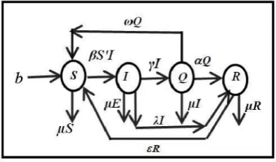
Fig. 3.1.Transition relationship of node states
Table 3.1 Parameters Used
S.No Symbol Meaning of Symbol
1 S Susceptible
2 I Infected
3 Q Quarantined
4 R Recovered
5 b Birth rate
6 µ Death rate
7 β Rate of infection
8 α Probability of moving from exposed node to
infec-tious category
9 γ Recovery rate of an infectious node
10 ω Probability of moving from Quarantined node to
Sus-ceptible node
11 ε probability at which a recovered node become a
sus-ceptible node
been considered in proposed model. A SIRS model was proposed by [33] in which consider the communication radius and node density as well as calculate the reproductive number and found the Eigen values for stability verification of the system. But this model have not efficient mechanism to control the quick spreading of worm in the network. We extend the proposed model with introduction of quarantined class. The quarantined state plays a significant role and sends the infectious nodes into isolation mode and removes the worm from network without any overhead and stretch the life span of network. This model overcomes the insufficiency of existing models.
4. Modeling and Analysis. We assume that the communication area of a sensor node is πr2 and the density of a susceptible node in a unit area is ρ(t) = S(t)/(L×L) . The total number of neighboring nodes which lie in the communication range of a sensor node is given as : S′(t) =ρ(t)πr2 = S(t)πr
2
L×L . According to Fig 3.1, we consider following mathematical model of worm propagation.
dS dt =b−
πr2
L2βSI+ωQ+εR−µS dI
dt = πr2
L2 βSI−(µ+λ+γ)I dQ
dt =γI−(α+ω+µ)Q dR
dt =αQ+λI−(µ+ε)R (4.1)
Letζ= πr 2
L2β. Then the above system (4.1) can be written as: dS
dt =b−ζSI+ωQ+εR−µS dI
dt =ζSI−(µ+λ+γ)I dQ
dt =γI−(α+ω+µ)Q dR
dt =αQ+λI−(µ+ε)R (4.2)
5. Existence of positive equilibrium. For equilibrium points we have dS
dt = 0, dI dt = 0,
dQ dt = 0,
dR dt = 0
and after a straight forward calculation, we get equilibrium points as P0 = (S0, I0, Q0, R0) = ( b
N,0,0,0) for worm free state andP∗= (S∗, I∗, Q∗, R∗) for endemic state, where
S∗= λ+γ+µ
ζ I
∗= (1− 1
R0
)b(ε+µ)(µ+α+ω)
A , Q
∗= (1− 1
R0
)γ(ε+µ) A , R
∗= (1− 1
R0
)α(γ+λ) +λ(µ+ω) A
where A = (µ+α)(λ+µ) + (µ+ε) + (γ+ε+ω) + (αγ+ωλ) and R0 [34] is the basic reproduction number and given byR0=
bζ
µ(µ+λ+γ). It is clear thatP
∗ exist and unique if and only ifR0 >1.
5.1. Stability analysis of the worm free equilibrium.
Theorem 5.1. The worm free equilibrium (W F E) is locally asymptotically stable if
R0 <1 otherwise unstable forR0 >1.
Proof. In order to check the stability of point ,we will find all the Eigenvalue values of the variational matrix is given by
J(P0) =
−ζI0−µ ζS0 ω −ε
ζI0 ζS0−(λ+γ+µ) 0 0
0 γ −(α+µ+ω) 0
0 0 α −(ε+µ)
Eigen values of (5.1) are: θ1=−µ,θ2=−(µ+α+ω),θ3= (ε+µ),θ4= (R0−1)( 1 γ+λ+µ).
It is clear that all eigen values of the variational matrix are negative whenR0<1. Therefore,the system is locally asymptotically stable at worm free equilibrium.Furthermore, the following theorem holds.
Theorem 5.2. The worm free equilibrium is said to be globally asymptotically stable ifR0≤1.
Proof. Consider the Lyapunov functionL(t): R4−→R+defined byL(t) =ηI(t),now taking time derivative ofL(t) with respect to timetis dL(t)
dt =η1I(t)⇒ dL(t)
dt =η(ζSI)−(γ+µ+λ)I) =η(ζS−(γ+µ+λ))I. After suitable assumption ofη= 1
(γ+λ+µ) we get dL
dt = [ζS−(γ+λ+µ] = [
ζb
(µ+γ+λ)µ−1]I= (R0−1)I. It is clear that dL
dt = 0 only whenI= 0. Therefore,the maximum invariant set Γ = (S, I, Q, R)∈R +
4 is the singleton set. Therefore, the global stability of worm free equilibrium P0 when R0 ≤1 follows from Lasalle invariance principle [35].
5.2. Stability analysis of Endemic equilibrium.
Theorem 5.3. Worm endemic state(WES)is locally asymptotically stable ifR0>1.
Proof. In order to check the stability at pointP∗we will find all the Eigen values of the variational matrix:
J(P∗) =
−ζI∗−µ ζS∗ ω ε
ζI∗ ζS∗−(λ+γ+µ) 0 0
0 γ −(α+µ+γ) 0
ω 0 0 −(ε+µ)
(5.2)
Therefore, the corresponding characteristic equation for the above matrix is given by
ν4+D1ν3+D2ν2+D3ν+D4= 0 (5.3)
where
D1=ζQ1(R0−1) + 3µ+α+ω+ε
D2= (µ+α+ω)(µ+ε) + (ζQ1((R0−1) +µ)(α+ 2µ+ω+ε) +Q2 D3=ζQ1(R0−1)(ωγ+ελ) + (µ+α+ω)(µ+ε)(Q2−1)
D4=ζQ1(R0−1)(γεα+ωγ(µ+ε) +Q3) where
Q1=
b(µ+α+ω)(µ+ε) AR0
, Q2=−ζ2I∗S∗,
Q3=−(α+µ+ω)[(µ+γ)(µ+ε) +µλ]
It is clear that all D1, D2, D3, D4 are positive when R0 >1,by a direct calculation G1 = D1 >0,G2 = D1D2−D3 > 0,G3 = D3G2−D21D4 >0 and G4 = D4, G3 > 0. Therefore, according to Routh Hurwitz criteria, all the roots of equation (5.3) have negative real parts. Therefore,the endemic equilibriumP∗is locally
asymptotically stable whenR0>1. This completes the proof.
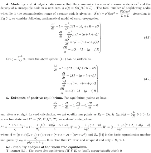
N= 1000;b= 1;L= 10;β= 0.0002;µ= 0.001;γ= 0.002;ε= 0.0003;ω= 0.0001;α= 0.002;λ= 0.0005;r= 0.7
Fig. 6.1.Dynamic behavior of model when communication radius is 0.7
6.1. Communication Radius of nodes r. As we have shown that
R0=
bζ
µ(µ+γ+λ), where ζ= πr2β
L2 .
From this equation, we find threshold radiusrc= L
√
(µ+γ+λ)µ π ¯β
i.e whenr≤rc, R0≤1 from theorem 5.2, it is clear that the worms in wireless sensor networks can be eradicated and system will stable at worm free equilibrium, when r > rc, R0 >1 according to theorem 5.3, worms in wireless sensor networks will be present consistently and system will stabilize at the endemic equilibrium.
We take following values of parameters as N = 1000;L= 10;b = 1;β = 0.0002;µ= 0.001;γ = 0.002;ε= 0.0003;ω = 0.0001;α = 0.002;λ = 0.0005. After calculation, we get rc = 0.746542 the initial values of
susceptible, exposed ,infected and recovered nodes in wireless sensor networks areS(0) = 990, I(0) = 10, Q(0) = 0 and R(0) = 0 and takes different values ofr, simulation results are described in Fig.6.1, 6.2 and 6.3. When r= 0.7< rc, Fig.6.1 shows that system (4.2) stabilizes at worm free equilibrium and the simulation results are
consistent with theorem 5.2.
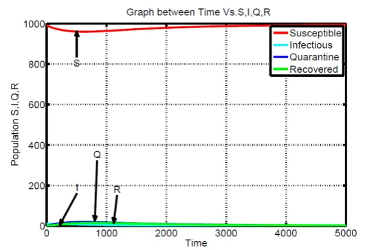
Whenr= (1.0 and 1.4)> rc, Figs. 6.2 and 6.3 shows that system (4.2) stabilizes at the endemic equilibrium
and the simulation results are consistent with theorem 5.3. Communication radius plays an important role for connectivity. Therefore, connectivity is a function of communication radius. From Figs. 6.1, 6.2 and 6.3 we see that when communication radius of nodes increases connectivity increases but the value of R0 also increases. When the communication radius less than rc the network will be stable and worm free. As the communication
radius increases R0 also increases and lead to the failure of the system.
Fig. 6.4 shows that relation between infected and recovered nodes with variation in the parameters. We observed that when the value ofαincreases the more number of nodes are recovered smoothly. We also find that if we increase the value of γ, less number of nodes get infected and recovered in short time. This experiment shows the effect of quarantined state on sensor network.
N= 1000;b= 1;L= 10;β= 0.0002;µ= 0.001;γ= 0.002;ε= 0.0003;ω= 0.0001;α= 0.002;λ= 0.0005;r= 1.0
Fig. 6.2.Dynamic behavior of model when communication radius is 1.0
N= 1000;b= 1;L= 10;β= 0.0002;µ= 0.001;γ= 0.002;ε= 0.0003;ω= 0.0001;α= 0.002;λ= 0.0005;r= 1.4
Fig. 6.3.Dynamic behavior of model when communication radius is 1.4
6.2. Node distributed density. The threshold value of node densityρthis given by
ρth=
N(µ+γ+λ)µ bπr2β
i.e., when ρ≤ ρth, R0 ≤ 1 then the system has only equilibrium and is globally asymptotically stable; when ρ > ρth, R0>1,system has only one endemic equilibrium which is locally asymptotically stable.
We take following values of parameter- N = 1000;b= 1;β = 0.0002;µ= 0.001;γ= 0.002;ε= 0.0003;ω = 0.0001, α = 0.002;λ = 0.0005;r = 1. After calculation ,we get ρth = 5.573248. Initial values of susceptible,
exposed ,infected and recovered nodes in wireless sensor networks are S(0) = 990, I(0) = 10, Q(0) = 0 and R(0) = 0 and WhenL= 11.18 and 8.45 ,we can getρ= 8 and 14 using these various values, simulation results are shown in Figs. 6.6 and 6.7. Whenρ=< ρth, the system (4.2) stabilizes at worm free equilibrium and the
N= 1000;b= 1;L= 10;β= 0.0002;µ= 0.001;γ= 0.002;ε= 0.0003;ω= 0.0001;α= 0.002;λ= 0.0005;r= 1.4
N= 1000;b= 1;L= 10;β= 0.0002;µ= 0.001;γ= 0.003;ε= 0.0003;ω= 0.0001;α= 0.003;λ= 0.0005;r= 1.4
N = 1000;b= 1;L= 10;β= 0.0002;µ= 0.001;γ= 0.0035;ε= 0.0003;ω= 0.0001;α= 0.004;λ= 0.0005;r= 1.4
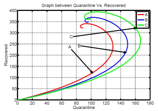
Fig. 6.4.Plot between Infected and Recovered
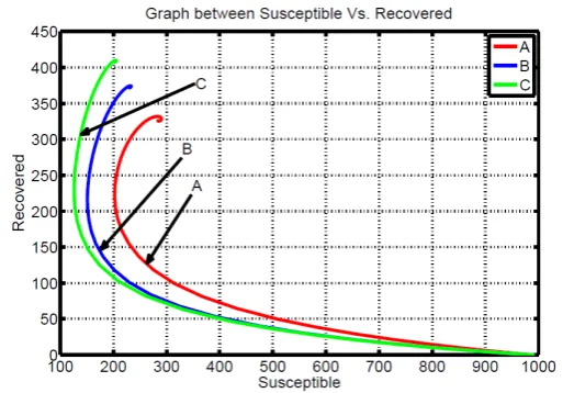
N= 1000;b= 1;L= 10;β= 0.0002;µ= 0.001;γ= 0.002;ε= 0.0003;ω= 0.0001;α= 0.002;λ= 0.0005;r= 1.4
N= 1000;b= 1;L= 10;β= 0.00024;µ= 0.001;γ= 0.003;ε= 0.0002;ω= 0.00014;α= 0.0024;λ= 0.0004;r= 1.4
N= 1000;b= 1;L= 10;β= 0.00028;µ= 0.001;γ= 0.0035;ε= 0.00025;ω= 0.00018;α= 0.003;λ= 0.0005;r= 1.4
Fig. 6.5. Plot between Susceptible and Recovered
and 6.7 again shows that the trajectories converge to the endemic equilibrium and the simulation results are consistent with the theoretical analysis.
Node density also affects the connectivity of wireless sensor network. From Figs. 6.6 and 6.7 when node density increases connectivity increases and value of R0 also increases. When the node density less than ρth= 7.043116 worm do not persist in the network. When the node density increasesR0also increases and this is harmful for network.
N= 1000;ρ= 8;b= 1;β= 0.0002;µ= 0.001;γ= 0.002;ε= 0.0003;ω= 0.0001α= 0.002;λ= 0.0005;r= 1
Fig. 6.6.Dynamic behavior of model when node density is 8.0
N = 1000;ρ= 14;b= 1;β= 0.0002;µ= 0.001;γ= 0.002;ε= 0.0003;ω= 0.0001α= 0.002;λ= 0.0005;r= 1
Fig. 6.7.Dynamic behavior of model when node density is 14.0
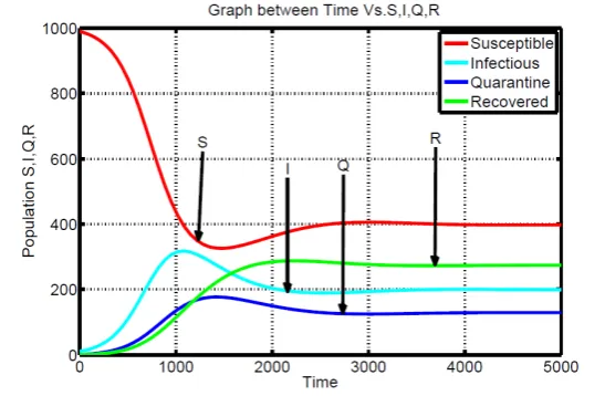
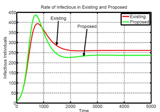
increased,the number of infectious nodes also increased. When λincreased and the remaining parameters are fixed number of recovered nodes increased. It is also found that,as time passes the number of infectious nodes increases and reached at maximum value at a certain stage this will depends on the parameters. Fig. 6.12 shows the comparison between [33] and proposed model. The plot shows that the proposed model is better in comparison to the existing model because more number of nodes are infected in existing model.
N= 1000;β= 0.0003;µ= 0.001;γ= 0.002;ε= 0.0003;ω= 0.0001;α= 0.004;λ= 0.0003;r= 1.4;ρ= 4.917
N= 1000;β= 0.00035;µ= 0.001;γ= 0.0023;ε= 0.0003;ω= 0.00014;α= 0.0045;λ= 0.00034;r= 1.4;ρ= 4.917
N = 1000;β= 0.0004;µ= 0.001;γ= 0.003;ε= 0.0003;ω= 0.00018;α= 0.005;λ= 0.0005;r= 1.4;ρ= 4.917
Fig. 6.8.Plot between Time and Infected nodes when node density is 8
N= 1000;β= 0.0003;µ= 0.001;γ= 0.002;ε= 0.0003;ω= 0.0001;α= 0.004;λ= 0.0003;r= 1.4;ρ= 4.917
N= 1000;β= 0.0003;µ= 0.001;γ= 0.002;ε= 0.0003;ω= 0.00014;α= 0.0045;λ= 0.0003;r= 1.4;ρ= 4.917
N = 1000;β= 0.0003;µ= 0.001;γ= 0.003;ε= 0.0003;ω= 0.00018;α= 0.005;λ= 0.0003;r= 1.4;ρ= 4.917
Fig. 6.9.Plot between Time and Quarantine nodes when node density is 4.917
number. Furthermore, we have done the simulation of proposed model with the help of MATLAB to verify and validate the results of proposed model. We study the impact of various parameters under different conditions. This model helps to developing an anti-virus mechanism for WSNs. Heterogeneous and moving nodes can be included for analysis of the model in future.On the basis of analysis worm riddance technique can be suggested.
REFERENCES
N= 1000;b= 1;L= 10;β= 0.0002;µ= 0.001;γ= 0.002;ε= 0.0003;ω= 0.0001;α= 0.002;λ= 0.0005;r= 1.4
N= 1000;b= 1;L= 10;β= 0.00028;µ= 0.001;γ= 0.002;ε= 0.0003;ω= 0.0001;α= 0.0024;λ= 0.00056;r= 1.4
N = 1000;b= 1;L= 10;β= 0.00035;µ= 0.001;γ= 0.002;ε= 0.0003;ω= 0.0001;α= 0.003;λ= 0.0006;r= 1.4
Fig. 6.10. Plot between Time and Infected nodes with variation of parameters
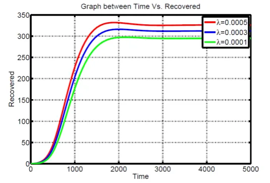
N= 1000;b= 1;L= 10;β= 0.0002;µ= 0.001;γ= 0.002;ε= 0.0003;ω= 0.0001;α= 0.002;λ= 0.0005;r= 1.4
N= 1000;b= 1;L= 10;β= 0.0002;µ= 0.001;γ= 0.002;ε= 0.0003;ω= 0.0001;α= 0.002;λ= 0.0003;r= 1.4
N= 1000;b= 1;L= 10;β= 0.0002;µ= 0.001;γ= 0.002;ε= 0.0003;ω= 0.0001;α= 0.002;λ= 0.0001;r= 1.4
Fig. 6.11.Plot between Time and Recovered nodes with variation of parameters
[2] S. Fedor and M. Collier,On the problem of energy efficiency of multi-hop vs one-hop routing in Wireless Sensor Net-works,in Proceedings of the 21st International Conference on Advanced Information Networking and Applications Work-shops/Symposia (AINAW 07), pp. 380385, May 2007.
[3] H. Shi, W. Wang, and N. Kwok,Energy dependent divisible load theory for wireless sensor network workload allocation, Mathematical Problems in Engineering, vol. 2012, Article ID 235289,16 pages,2012.
[4] J.Zhang and H.-N.Lee,Energy-efficient utility maximization for wireless networks with/without multipath routing, AEU International Journal of Electronics and Communications,vol. 64,no.2,pp. 99111,2010.
[5] H. Chen, C. K. Tse, and J. Feng,Impact of topology on Performance and energy Efficiency in wireless sensor networks for source extraction,IEEE Transactions on Parallel and Distributed Systems,vol.20,no.6,pp.886897,2009.
N= 1000;b= 1;L= 10;β= 0.0002;µ= 0.001;γ= 0.002;ε= 0.0003;ω= 0.0001;α= 0.002;λ= 0.0005;r= 1.4
Fig. 6.12.Plot between Time Vs. Infected nodes For Existing and Proposed model
no.4, pp. 795-806, 2009.
[7] M.H.Khouzani and S.Sarkar,Maximum damage battery depletion attack in mobile sensor networks,IEEE Transactions on Automatic Control, vol. 56, no. 10, pp. 2358-2368, 2011.
[8] P. De, Y. Liu, and S.K. Das,An epidemic theoretic framework for vulnerability analysis of broadcast protocols in wireless sensor networks,IEEE Transactions Mobile Computing, vol. 8, no. 3, pp. 413-425, 2009.
[9] S.Zanero,Wireless malware propagation:a reality check,IEEE Security & Privacy, vol. 7, no. 5, pp. 70-74, 2009.
[10] Shensheng Tang,A Modified SI Epidemic Model for Combating Virus Spread in Wireless Sensor Networks.Int J Wireless Inf Networks (2011) 18:319326.
[11] J.L. Sanders,Quantitative guidelines for communicable disease control programs, Biometrics, Vol. 27, pp. 883-893, 1971. [12] R.Pastor-Satorras and A.Vespignani,Epidemic spreading in scale free networks, Physical Letters, Vol. 86, pp. 3200-3203,
2001.
[13] Y. Moreno, M. Nekovee, and A.Vespignani,Efficiency and reliability of epidemic data dissemination in complex networks, Physical Review E, Vol. 69, pp. 1-4, 2004.
[14] A. Khelil, C. Becker, J. Tian, and K. Rothermel,Directed-graph epidemiological models of computer viruses. In Proc. 5th ACM Intl Workshop on Modeling Analysis and Simulation of Wireless and Mobile Systems, pp. 54-60, 2002. [15] H. Zheng, D. Li, and Z. Gao,An epidemic model of mobile phone virus. In 1st Intl Symposium on Pervasive Computing
and Applications, pp. 1-5, 2006.
[16] S.K.Tan and A.Munro,Adaptive probabilistic epidemic protocol for wireless sensor networks in an urban environment. In Proc. 16th International Conference on Computer Communications and Networks (ICCCN 2007), pp. 1105-1110, 2007. [17] J. Kim, S. Radhakrishnan, S.K. Dhall,Measurement and analysis of worm propagation on Internet network topology, Proc.
of IEEE International Conference on Computer Communications and Networks, Chicago, Illinois, USA, pp.495-500, 2004. [18] C.C. Zou, W. Gong, D. Towsley,The monitoring and early warning for Internet worms, IEEE Transactions on Networking,
Vol. 13, No. 5, pp. 961-974, 2005.
[19] J.C. Frauenthal,Mathematical Modeling in Epidemiology, Springer-Verlag, New York, USA,1980.
[20] D. Moore, V. Paxson, S. Savage, C. Shannon,S. Stanoford ,N. Weaver,Inside the slammer worm, IEEE Security & Privacy, Vol.1, No.4, pp. 33-39, 2003.
[21] R. Dantu, J.W. Cangussu, S. Patwardhan,Fast worm containment using feedback contro, IEEE Transactions on Depend-able and Secure Computing, Vol. 4, No. 2, pp. 119-136, 2007.
[22] Zhang Shu-kui, Gong Sheng-rong, Cui Zhi-ming, Study On Spreading of Virus infection with SIRS characteristic in Wireless Sensor Network, Proceeding of International Conference on Communication and Mobile Computing, 12-517, 2009.
[23] Roberto Di Pietro, Nino Vincenzo Verde,Introducing Epidemic Models for Data Survivability in Unattended Wireless Sensor Networks, Proceeding of 4th ACM Conference on Wireless Network Security (WiSec11), pp.11-22, 2011. [24] Wang Ya-Qi, Yang Xiao-Yuan,Virus spreading in wireless sensor networks with a medium access control mechanism. Chin.
Phys. B, 22(4), 040206, 2013.
[25] S.Tang, Brian L.Mark,Analysis of Virus Spread in Wireless Sensor Networks: An Epidemic Model, Design of Reliable Communication Networks pp. 86- 91, 2009.
[26] X.M. Wang and Y. S. Li, An improved SIR model for analyzing the dy namics of worm propagation in wireless sensor networks,Chinese Journal of Electronics, vol. 18, no. 1, pp. 8-12, 2009.
Stability Analysis of SIDR Model for Worm Propagation in Wireless Sensor Network, Indian Journal of Science and Technology, Vol 9(32),2016.
[28] Linhe Zhu and Hongyong Zhao,Dynamical analysis and optimal control for a malware Propagation model in an information network, Neurocomputing (2014).
[29] A. Martn del Rey, A.Hernndez Encinas, J.D.Hernndez Guilln, J.Martn Vaquero, A. Queiruga Dios and G. Ro-drguez Snchez,An Individual-Based Model for Malware Propagation in Wireless Sensor Networks, DCAI, 13th Inter national Conference (2016),Advances in Intelligent Systems and Computing 474, pp. 223-230.
[30] Rudra Pratap Ojha, Pramod Kumar Srivastava, Shashank Awasthi and Goutam Sanyal,Global Stability of Dynamic Model for Worm Propagation in Wireless Sensor Network, Proceeding of International Conference on Intelligent Commu-nication, Control and Devices (ICICCD 2016), Advances in Intelligent Systems and Computing Volume 479, pp.695-704, 2017.
[31] Shensheng Tang, David Myers and Jason Yuan,Modified SIS epidemic model for analysis of virus spread in wireless sensor networks, Int. J. Wireless and Mo bile Computing, Vol. 6, No.2, 2013, pp.99-108.
[32] Keshri, N.; Mishra, B.K.,Two time-delay dynamic model on the transmission of malicious signals in wireless sensor network. Chaos Solitons Fractals, 68, 51158, 2014.
[33] Liping Feng, Liping Song, Qingshan Zhao, Hongbin Wang,Modelling and Stability Analysis of Worm Propagation in Wireless Sensor Network, Mathematical Problems in Engineering 2015.
[34] Driessche,P.V. and Watermouch, J,Reproduction number and sub- threshold endemic equlibria for compartmental models of disease transmission. Mathematical Biosciences, Vol. 180, pp. 29-48, 2001.
[35] LaSalle, J,The stability of dynamical systems. Regional to conference series in applied mathematics, pp. 96-106, 1976.
Edited by: Gulshan Shrivastava
Received: May 25, 2017