Scalable Computing: Practice and Experience
Volume 17, Number 1, pp. 13–32. http://www.scpe.org
ISSN 1895-1767 c
⃝2016 SCPE
USING COMPUTATIONAL GEOMETRY TO IMPROVE PROCESS RESCHEDULING ON ROUND-BASED PARALLEL APPLICATIONS
RODRIGO DA ROSA RIGHI, VLADIMIR MAGALH ˜AES GUERREIRO, GUSTAVO ROSTIROLLA, VINICIUS FACCO RODRIGUES, CRISTIANO ANDR´E DA COSTA AND LEONARDO DAGNINO CHIWIACOWSKY ∗
Abstract. Process rescheduling is a known technique to face with system heterogeneity and dynamism, being especially pertinent on Bulk Synchronous Parallel (BSP) programs. These programs are organized in a set of round-based supersteps, in which the slowest process determines the moment of synchronization. This approach motivated us to develop a first model called MigBSP, which combines computation, communication and migration costs metrics for process rescheduling decisions. MigBSP originally employed an heuristic that could select either a single or a collection of process to migrate at each load balancing invocation. The first proposal is not reactive, so you should manually setup a percentage of processes to be migrated as input parameter for the load balancing model. In this work, two novel heuristics, named MigCube and MigHull, are proposed to choose the candidate processes for migration and their destination. Both heuristics consider the use of computational geometry for plotting computation, communication and migration costs metrics in a 3D graph, so both ‘which’ and ‘where’ load balancing questions can be answered without any user intervention. We believe that the contribution is not only in the MigBSP landscape, but also for the BSP community, who is trying to enhance performance in round-based applications in an effortless way. In addition to the description of MigCube and MigHull, this article also presents their evaluations with performance gains of up to 42% when enabling process migration over a subset of the Grid5000 infrastructure.
Key words: Computational Geometry, Process Migration, Performance, Dynamism, Grid Computing
AMS subject classifications. 15A15, 15A09, 15A23
1. Introduction. Process migration is a useful mechanism to offer runtime load balancing, mainly in dynamic, complex and heterogeneous environments. Generally, process migration requires explicit rescheduling calls within the application [11]. A different migration approach happens at middleware level, where changes in the application code and previous knowledge about the system are usually not required. Considering this, we have developed a process rescheduling model for grid computing architectures called MigBSP [28]. We decided to work with round-based applications, such as those that follow the BSP (Bulk-Synchronous Parallel) programming model [33]. Concerning the choose of migration processes, MigBSP creates a priority list based on the highest Potential of Migration (PM) of each process. PM is a decision function that combines the migration costs with data from computation and communication phases in order to create a unified scheduling metric.
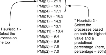
Taking profit from the highest PM of each process, MigBSP could originally employ one of two methods to select the candidate processes for migration. As illustrated in Figure 1.1, MigBSP can select one or a group of processes located on the top of the list. The second case is viable thanks to a predefined percentage that acts over the highest PM value. Although we achieved good results particularly with this second approach [28], we agree that the use of another percentage value could eventually determine better migration results. Consequently, a question arises: Using the PM idea, how can one reach an optimized percentage of migratable candidates on dynamic environments? A solution involves the testing of several hand-tuned parameters for each new BSP application and a comparison among the results.
After developing the first version of MigBSP, we focused our research on investigating new heuristics and metaheuristics in order to fill the aforementioned gap. We followed this rationally because both scheduling and rescheduling techniques are classified as NP-hard problems [15]. Taking into account metaheuristics, Genetic Algorithms [14, 22, 26], Simulated Annealing [13, 34], Artificial Bee Algorithms [16, 3], Pareto Search [32] and Hybrid Schemes [18] are commonly used for these tasks. Considering their iterative nature, they are known by reaching high-quality solutions meanwhile paying a high-computational time for achieving optimal or near-optimal solutions. On the other hand, heuristics are faster than metaheuristics, since they operate with mental shortcuts to ease the cognitive load of making a decision [9]. Thus, heuristics such as min-min and max-min operate by trading optimistically, completeness, accuracy, or precision for speed. When analyzing the state-of-the-art on migration-aware BSP communication libraries [8, 19, 21, 24, 25, 28, 35], we still observe that both
∗Applied Computing Graduate Program, Universidade do Vale do Rio dos Sinos, S˜ao Leopoldo - Rio Grande do Sul - Postal
Code 93022-000 - Brazil ([email protected]).
PM(p7) = 21.3 PM(p3) = 19.5 PM(p4) = 17.1 PM(p10) = 16.2 PM(p1) = 14.3 PM(p6) = 13.1 PM(p11) = 10.4 PM(p8) = 9.4 PM(p9) = 8.9 PM(p5) = 7.6 PM(p2) = 7.0 * Heuristic 1 -
Select the process on the top
* Heuristic 2 - Select the processes based on both the highest value and a predefined percentage (here, percentage = 80%)
Fig. 1.1: Current MigBSP’s methods for choosing the candidate processes for migration based on a decision function named Potential of Migration (PM).
heuristics and metaheuristics techniques are not employed to offer rescheduling under the following constraints: (i) combination of multiple metrics; (ii) automatic selection of candidate processes for migration without user intervention.
When process (re)scheduling is considered, two timers are involved: calculus complexity and quality of the mapping. Both measures are used in heuristics for optimizing the MigBSP’s initial approaches. In this regard, we developed two novel heuristics named MigCube and MigHull for automatically selecting one or more candidates for migration at each rescheduling attempt. They solve a 3D geometric query problem taking profit from the computation, communication and migration costs metrics of the PM as the values for the x, y and z axes. So, the scientific contribution of the article consists in exploring computational geometryconcepts to select the most suitable points arranged in a three-dimensional space, consequently indicating the processes for migration, without needing any intervention when considering the user viewpoint. MigCube explores the Euclidean distance [12] among the points while MigHull extends the idea of Convex Hull for a 3D setting [4].
This article presents the algorithms of MigCube and MigHull in detail, followed by their evaluation when using two BSP scientific applications over a subset of the Grid5000 infrastructure1. Besides not needing a
particular parameter in the model at compilation time, the results also show the benefits of selecting a more appropriate number of migratable processes instead of selecting just one or a percentage of them. The contri-bution of both proposed heuristics does not appear only in the MigBSP scope, but also for the BSP community who is interested in efficient migration process at middleware level in an effortless way.
The remainder of this article will first introduce the fundamental concepts in Section 2, explaining how MigBSP works in detail. The main part of the paper belongs to Section 3, where both MigCube and MigHull algorithms are proposed. Sections 4 and 5 show the employed methodology and the results, respectively. Related work is discussed in Section 6. Finally, Section 7 emphasizes the scientific contribution of the work and notes challenges that we can address in the future.
2. Fundamental Concepts. This section explains the functioning of MigBSP, emphasizing its rationales and parameters. MigBSP is a rescheduling model that works over heterogeneous resources, joining the power of clusters, supercomputers and local networks. The heterogeneity issue considers the processor’s clock (all processors have the same set of instructions), as well as the network bandwidth. Such an architecture is assembled with Sets (sites or clusters) and Set Managers. Set Managers are responsible for scheduling, capturing data from a Set and exchanging it among other managers [28].
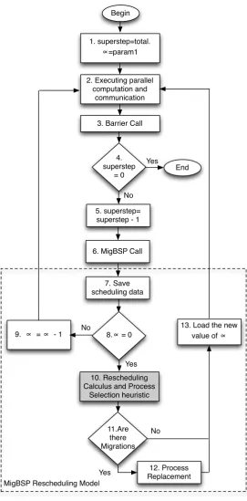
The decision for process remapping is taken at the end of a superstep. A BSP program has an arbitrary number of supersteps, each one composed by a local computation phase on each process, a global and arbitrary communication phase among the processes and a synchronization barrier [33]. Aiming at not trying to test process rescheduling at each conclusion of superstep, we designed a parameter namedαto control the interval of supersteps between two consecutive attempts for process rescheduling. Thus, we applied two adaptations
1
that control the value of the α(α∈N) in order to reduce the scheduling model intrusiveness: (i) to postpone the rescheduling call if the processes are balanced or to turn it more frequent, otherwise; (ii) to delay this call if a pattern without migrations onω past calls is observed. Thus,αis automatically updated at each rescheduling call and will indicate the interval for the next one (more details in [28]). A shorter initial value ofαwill bring better reactivity on application reorganization, since process rescheduling will be evaluated as soon reaching the αthsuperstep. So, this configuration implies on reconfiguring the application sooner, benefiting the remaining of the execution with an optimized process-resources mapping. However, if process migration is inviable (due to the large number of bytes to be transferred or a prohibitive network latency overhead, for example), a shorter αwill cause more overhead in the normal execution of the application. In this last case, process rescheduling is tested more frequently, but no migrations take place actually.
The answer for ‘Which’ is solved through our decision function called Potential of Migration (PM). Each processicomputesnfunctionsP M(i, j), wherenis the number of Sets andj means a particular Set. The key rationale consists in performing only a subset of the processes-resources tests at the rescheduling moment. The value ofP M(i, j) is found using Computation, Communication and Memory metrics as presented in Equations 2.1–2.4. A previous paper describes them in detail [28]. The greater the value ofP M(i, j), the more prone the processes will be to migrate.
Comp(i, j) =Pcomp(i)×CT Pk+α−1(i)×ISetk+α−1(j); (2.1)
Comm(i, j) =Pcomm(i, j)×BT Pk+α−1(i, j); (2.2)
M em(i, j) =M(i)×T(i, j) +M ig(i, j); (2.3)
P M(i, j) =Comp(i, j) +Comm(i, j)−M em(i, j). (2.4)
Computation metric Comp(i, j) considers a Computation Pattern P comp(i) that measures the stability of a process i regarding the number of instructions at each superstep. This value is close to 1 if the process is regular and close to 0 otherwise. Furthermore, we also have a computation time prediction CT P(i) for process i based on all computation phases between two rescheduling activation. In this way, here k refers to the index of the last call for process rescheduling and k+α−1 means the interval of supersteps from the last to the current rescheduling attempt. The metric Comp(i, j) also presents an indexISet(j) which informs the average computation capacity of Setj. In the same way, Communication metricComm(i, j) computes the Communication PatternP comm(i, j) between processes and Sets. Furthermore, this metric uses communication time predictionBT P(i, j) considering data between two re-balancing activation. Comm(i, j) increases if process ihas a regular communication with processes from Setjand performs slower communication actions to this Set. The metric M em(i, j) considers process memory M(i), transferring rateT(i, j) between considered process i and the manager of target Setj, as well as migration costsM ig(i, j). These costs are dependent of the operating system, as well as the migration tool [28].
At each rescheduling call, each process passes its highest P M(i, j) to its Set Manager. This last entity exchanges the PM of the processes with other managers. As described earlier, each manager creates a decreasing-sorted list and selects either the process on the top or a percentage of them for testing the migration viability. Here, besides using the abstraction of Set, this test also considers the following data: (i) the external load on source and destination processors; (ii) the processes that both processors are executing; (iii) the simulation of considered process running on a destination processor; (iv) the time of communication actions considering local and destination processors; (v) migration costs. We used these five information to compute the migration viability of each process through a relationship between two timers: t1 andt2. t1 means the superstep time of processiin the current processor, whilet2 encompasses its execution on the other processor and it includes the migration costs. Process migration takes place ift1> t2.
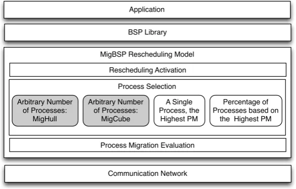
applications at the rescheduling moment. The main idea is to outperform the current MigBSP strategies for this task, particularly without user intervention at editing or launching time to set model parameter for selection purposes. At the application perspective, the use of a particular selection policy or even process rescheduling facility is totally hidden from the user. Usually, for the submission of a BSP application in a grid, it is previously compiled with a rescheduling-aware BSP library, informing an initial processes-nodes scheduling [38]. Figure 3.1 depicts the software stack when using MigBSP. The gray boxes represent the scope of this article.
Application
BSP Library
MigBSP Rescheduling Model
Process Selection
A Single Process, the
Highest PM
Percentage of Processes based on
the Highest PM Arbitrary Number
of Processes: MigCube Arbitrary Number
of Processes: MigHull
Communication Network Rescheduling Activation
Process Migration Evaluation
Fig. 3.1: Software stack when using the novel heuristics for BSP process rescheduling
BSP applications have their performance always driven by the slowest process, so both heuristics try to optimize the number and the selection of processes to eventually migrate so that the remaining supersteps may run faster. Unlike previous approaches, MigCube and MigHull select an arbitrary number of processes but also considering the list of the highest PM of each process. Figure 3.2 illustrates the rescheduling in a BSP application. The mapping quality of MigCube or MigHull will impact the next value ofα parameter. If the system is classified as balanced, the value of αis increased in order to postpone the next call for process rescheduling.
Both MigCube and MigHull take profit from the list of the highest PM of each process. Considering that each PM identifies a process and a target Set, and since all the three assumed metrics are expressed in the same data unit, we may plot them as a single point in a 3D setting. In this way, the proposed heuristics must answer the following answer: Which points should be selected at each rescheduling call? To accomplish this, MigCube and MigHull use computational geometry to analyze a set of points, in order to efficiently find which points are close to the input query. At model level, each Set Manager compute the selected points locally, each one referring to a particular process i that presents a P M(i, j). After that, only the source and the target Sets (represented byjin theP M notation) are involved to transfer a processiactually. The destination Set informs the source Set about which is the most suitable processor under its responsibility to receive the process.
1. superstep=total.
∝
=param1Begin
End 2. Executing parallel
computation and communication
3. Barrier Call
4. superstep
= 0
9.
∝
=∝
- 15. superstep= superstep - 1
8.
∝
= 010. Rescheduling Calculus and Process
Selection heuristic
11.Are there Migrations
12. Process Replacement
13. Load the new
value of
∝
Yes
No
Yes
No
MigBSP Rescheduling Model
6. MigBSP Call
7. Save scheduling data
Yes No
Cube
x y
z
p1
p1 = Process with the Largest PM
Remaining BSP processes
Region indicating the candidate processes for migration
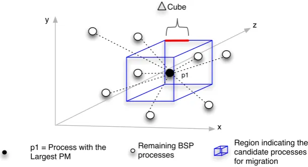
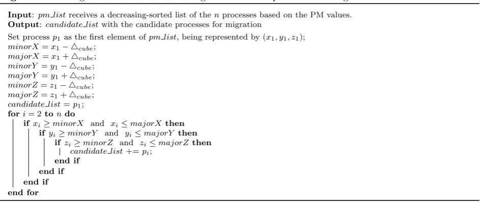
Fig. 3.3: Processes and cube representation in MigCube heuristic. Those processes that are located inside the cube will be appointed as candidate processes for migration.
such as Simulated Annealing, Tabu Search, Genetic Algorithms and Swarm Intelligence Schemes, needing only a given quality measurement to be performed.
3.1. Terminologies. Both MigCube and MigHull plot each process pi (i= 1,2, . . . , n) as a point in the 3D Cartesian coordinate system where xi, yi and zi represent the coordinates ofpi on each of the graph axes. Here, xi,yi andzi also represent respectively, the computation, communication and memory metrics from the largest PM of pi. In addition, a processpi can be also represented aspi= (xi, yi, zi).
3.2. MigCube Heuristic. MigCube uses the processes’ location to create a cube, so selecting as candi-dates those processes inside it. The algorithm starts by selecting the central point of the cube, which refers to the point that has the largest PM. Its notation isp1 and it represents the best candidate for migration. After
that, parameter △cube is computed in accordance with Equation 3.1 as an average of the distances from the aforementioned point to the others. Equation 3.2 computes the distance between p1 and any point pi in the 3D coordinate system. Finally,△cube is used to situate the cube edges as defined in Equation 3.3.
△cube= 1 n−1
n ∑
i=2
D(p1, pi) ; (3.1)
D(p1, pi) = 2 √
(x1−xi)2+ (y1−yi)2+ (z1−zi)2; (3.2)
edge= 2△cube. (3.3)
Figure 3.3 depicts an example of the points and the cube, wherep1has the largest PM. Algorithm 1 presents
Algorithm 1:MigCube heuristic for selecting the candidate processes for migration. Input:pm listreceives a decreasing-sorted list of thenprocesses based on the PM values. Output:candidate listwith the candidate processes for migration
Set processp1as the first element ofpm list, being represented by (x1, y1, z1);
minorX=x1− △cube; majorX=x1+△cube; minorY =y1− △cube; majorY =y1+△cube; minorZ=z1− △cube; majorZ=z1+△cube; candidate list=p1; fori= 2tondo
if xi≥minorX and xi≤majorX then
if yi≥minorY and yi≤majorY then
if zi≥minorZ and zi≤majorZthen candidate list+=pi;
end if end if end if end for
3.3. MigHull Heuristic. MigHull heuristic is a Convex Hull adaptation. In brief, the Convex Hull or Convex Envelope of a setSof points in the Euclidean plane is the smallest convex set that containsS[6, 4]. It can be seen as a convex polygon whose vertices are some of the points in the input set. MigHull employs the Convex Hull ideas, but providing two adaptations: (i) three-dimensional space is split in three two-dimensional planes; (ii) despite of selecting all processes, MigHull chooses only a part of them based on the two processes with the highest PM values.
We are calculating three 2D hulls, considering a pair of coordinates of each point iat a time, as follows: (i) xi and yi; (ii) xi and zi; and (iii) yi and zi. Figure 3.4 (a) illustrates this idea. Here, each process that is inside each plane concomitantly is then selected as a candidate for migration. For the standard 2D Convex Hull, the problem consists of finding the smallest convex polyhedron/polygon containing all the points. Thus, the native Convex Hull always selects all the points, which would not make sense for migration decision-making. In this way, we are adapting the QuickHull algorithm [5] to select processes. By default, QuickHull finds the points with the minimum and maximum xcoordinates and creates a line between them. The next step in the QuickHull algorithm is the selection of the point with the maximum distance from the aforesaid line, so the two points found before along with this one form a triangle. The points lying inside of that triangle cannot be part of the convex hull and can therefore be ignored in the next steps. Discarding the tested point and the previous ignored ones, the algorithm selects the next point with the maximum distance from the line and proceeds the same calculus again.
MigHull changes QuickHull as follows. Considering the plane a−b, whereameans the abscissa andbthe ordinate, we are considering the a-coordinate of the two points with the highest PM to draw a line segment between them. After that, we calculate △Hull as the maximum distance of coverage from this line segment to the other processes, so the processes inside this region are candidates to migrate in the scope of a−b plane. Figure 3.4 (b) illustrates an example of this procedure for the x−yplane, but the same is evaluated for other two planes: x−zandy−z. In other words, by substituting x−y plane byx−zandy−zthe distance△Hull is also calculated in the x−z and y−z planes, respectively. Finally, the processes that appear as candidates concomitantly in the x−y, x−z andy−z planes are selected as final candidates to migrate according to the MigHull algorithm.
△Hull=σ(x, y) =M ax(σ(x), σ(y)). (3.4)
x-z y-z
x-y
BSP Processes (a)
(b) Remaining BSP Processes x
y
Hull
p1 and p2: First and Second BSP Process with the Highest PM values
Region indicating the candidates for migration in the x-y plane p1
p2
Fig. 3.4: Selection of candidate process for migration with MigHull: (a) Creating three planes (x-y, x-z and y-z) from the three-dimensional space; (b) partially selecting the candidate process in the x-y plane. Those processes that appear concomitantly in the yellow region of the three planes are chosen for the next rescheduling step: the tests of migration viability.
considering the coordinate a. Using Figure 3.4 (b) as an example, we firstly take the value of the coordinatex of all the 11 points, computing the standard deviationσ(x) of these respective values. The same calculation is performed with respect to theyaxis, so the greatest standard deviation is selected as△Hullfor thex−yplane. In order to identify the candidate processes for migration, the distance of any point pm to the line determined by the pointsp1andp2over a specific plane (see Algorithm 2) is computed and denoted asd(pm, p1, p2, plane).
These last two points represent the processes with the highest PM. If x-coordinate ofpm is lower or greater than the x-coordinate of points used as limits of the line segment, we are computing the Euclidean distance given by the Pythagorean formula [12]. Otherwise, we are using the perpendicular distance from a point to a line determined byp1 andp2. Although Algorithm 2 was developed for thex-y plane, its use forx-zandy-zis
trivial and not explained here.
Figure 3.4 (b) depicts the MigHull ideas to create a region of candidate processes for migration. Contrary to MigCube, MigHull always selects at least two processes as candidates for migration: p1andp2. Independently of
Algorithm 2:Calculating the distanced(pm, p1, p2, plane) from the pointpmto the line segment created by the pointsp1 andp2 in thex−y plane.
Input:p1 (x1, y1, z1) andp2(x2, y2, z2) denote the two processes with the highest PM values. The pointpm(xm, ym, zm)
refers to one of the remaining processes, where 3≤m≤n.
Output: Distanced(pm, p1, p2, plane) from the pointpmto the line created byp1 andp2in the plane denoted byplane.
Denoteax+by+cas the line equation formed by the pointsp1andp2, where the coefficients are defined as:
a= (y1−y2),b= (x2−x1) andc= (x1y2−x2y1); if xm< x1 then
d(pm, p1, p2,“x−y”) =
√
(x1−xm)2+ (y1−ym)2
end if
else if xm> x2then
d(pm, p1, p2,“x−y”) =
√
(xm−x2)2+ (ym−y2)2 end if
else
d(pm, p1, p2,“x−y”) =
axm+bym+c √
a2 +b2 end if
Algorithm 3:MigHull heuristic for selecting the candidate processes for migration. Input:pm listreceives a decreasing-sorted list of thenprocesses based on the PM values. Output:candidate listwith the candidate processes for migration.
Set processesp1andp2 as the first and the second elements ofpm list, being represented by (x1, y1, z1) and (x2, y2, z2), respectively;
candidate list=p1;
candidate list+=p2;
candidatex-y = null;
candidatex-z = null;
candidatey-z = null; fori= 3tondo
if d(pi, p1, p2,“x−y”)≤ △H ull then candidatex-y +=pi;
end if end for
fori= 3tondo
if d(pi, p1, p2,“x−z”)≤ △H ullthen candidatex-z +=pi;
end if end for
fori= 3tondo
if d(pi, p1, p2,“y−z”)≤ △H ull then candidatey-z +=pi;
end if end for
candidate list+={candidatex-y∩candidatex-z∩candidatey-z}
p2 p3 p6 p4 p5
p7
(a) Crescent
(b) Decrescent
(c) CPU
(d) Round-Robin p1
p5 p6 p1 p2 p3
p7 p4
p5 p4
p2 p3
p1 p7
p6
p2 p3 p4 p5 p6
p7 p1
Cluster A has 3 nodes, each one with 500 MHz
A1
A1
A1
A1
A2 A3 B1 C1 C2
A2 A3 B1 C1 C2
A2 A3 B1 C1 C2
A2 A3 B1 C1 C2
Cluster B has 1 node with 1.5 GHz
Cluster C has 2 nodes, each one with 1.2 MHz
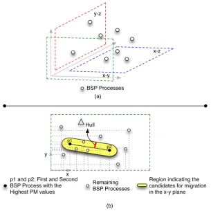
Fig. 4.1: Example of the four initial processes-resources scheduling employed in the tests using a hypothetical grid infrastrucuture.
comparison study among MigCube, MigHull and the originals heuristics of MigBSP, so we can analyze the impact of these values ofαon different algorithms for process migration.
Since the MigBSP was designed for grid environments, we are testing it with the proposed heuristics over the Grid5000 platform2. In fact, this platform is an XML file used by SimGrid, denoting machines, clusters and
network configurations. Besides the platform file, SimGrid also receives as input another XML file informing the first scheduling (deployment). Particularly, we are using 45 nodes, distributed in 3 distinct sites, each one offering here a single cluster. We are using the 10 nodes from cluster Chicon, 15 from cluster Capricorne and 15 nodes from cluster Suno. The hardware information is described as follow: (i) Chicon has AMD Opteron 2.6 GHz processors with 4GB of memory and a Gigabit Ethernet card; (ii) Capricorne has AMD Opteron 2.0GHz processors, with 2GB of memory and a Myrinet network card; (iii) Suno has Intel Xeon E5520 2.26GHz processors with 32GB of memory and 2 Gigabit Ethernet cards. Considering the deployment file, we are working with 60 processes that are launched in accordance with an initial process-scheduling mapping. We are considering four of them, explained below and detailed in the example of Figure 4.1:
(a) Ascending: Processes are scheduled cyclically in Ascending order of nodes’ processing power;
(b) Descending: Same idea of the Ascending mapping, but in reverse order, where the nodes with the higher
2
capacities are the first to receive processes;
(c) CPU: This mapping allocates each process to the resource that has the largest amount of free processing power on that moment;
(d) Round-Robin: It allocates the processes cyclically without taking into account any characteristics of the resources.
The initial mapping will influence the execution time directly, also influencing the rescheduling model in the same way. For example, the CPU mapping implies on using load balancing in accordance with the CPU power of the nodes, so this idea of equilibrium from the beginning tends to reduce the number of migrations at runtime. On the other hand, for example, the scheduling of all process in a single node could compromise the performance, imposing more rescheduling actions afterwards to spread them in the resource pool. Besides the initial mappings and MigBSP parameters, the tests also consider three scenarios: (i) execution of the native application, without MigBSP or proposed heuristics; (ii) the application runs with MigBSP, which performs the heuristics calculus and message-passing, but does not migrate any processes actually; (iii) the application runs with MigBSP and an heuristic to select the candidate processes for migration, enabling then any migration if it was evaluated as viable. The main idea is to show the overhead impact of the heuristic execution (comparison between scenarios (i) and (ii)) and performance impact when enabling migrations (comparison between scenarios (i) and (iii)).
Regarding the BSP application, we developed an implementation of the Lattice-Boltzmann method [29] to compute fluid dynamics. Technically, this method considers a typical volume of fluids composed of a collection of particles, where a particle is represented by a distribution function for each fluid component at each grid point. The data volume is divided into continuous blocks of equal size in accordance with the number of processes. Each block is copied and runs in a BSP process. After the computation phase, each process sends data to its right-sided neighbor. Finally, a synchronization barrier takes place and other superstep is computed afterwards. 5. Discussion of Results. The results consider the performance of MigCube and MigHull heuristics in terms of application processing time in Subsections 5.1 and 5.2. In addition, we also present two subsections, 5.3 and 5.4, for comparison purposes; the first one analyzes MigCube against MigHull and the second one compares both approaches with the standard process selection heuristics from MigBSP. We are using a BSP implementation of the fluid dynamics application with variations in the following configurations: number of supersteps; initial process-processor scheduling; the MigBSP’s parameter denoted α; and the aforementioned evaluation scenarios.
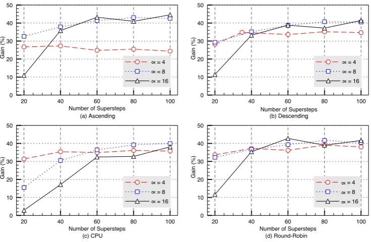
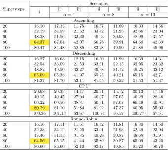
5.1. MigCube Evaluation. Table 5.1 shows the test results with MigCube. Scenario (ii) always produces a time larger than scenario (i), since the first adds the heuristic calculus and message passing. This overhead can be considered as part of the heuristic execution cost. The mean overhead of MigCube is 3.21%. This overhead also takes place when migration are enabled but any process replacement is viable during the application execution. The effectiveness of MigCube appears when comparing scenarios (iii) and (i). The larger the number of supersteps, the larger the gains with process migration. In other words, an application that migrates the processes in the first supersteps presents better performance because of both it has more time to amortize the penalties involved in process migration and more time to execute with an optimized configuration. The highlighted fields show that only one migration happens when using 20 supersteps andαequal to 16. Although achieving better results than scenario (i), the system remains unbalanced. This situation is only solved when 60 supersteps are performed.
Figure 5.1 shows the percentage of gain in execution time when analyzing scenarios (iii) and (i). It has been calculated using the following equation:
Gain = Scenario(i)−Scenario(iii)
Scenario(i) ×100. (5.1)
Table 5.1: MigCube evaluation. The times are expressed in seconds. We are highlighting the execution of 20 supersteps withα=16, where a single process migration takes place.
Supersteps
Scenarios
i ii iii ii iii ii iii
α= 4 α= 8 α= 16
Ascending
20 16.10 17.39 11.79 16.57 10.85 16.33 14.33
40 32.19 34.59 23.41 33.42 20.00 32.66 20.66
60 48.28 51.86 36.29 49.93 28.32 48.99 27.42
80 64.37 67.00 47.97 66.78 36.66 65.60 38.00
100 80.47 84.90 60.85 83.28 46.20 81.88 44.61
Descending
20 16.27 16.68 11.67 16.55 11.50 16.39 14.41
40 32.94 33.09 21.47 33.28 21.36 33.20 21.99
60 48.82 49.50 32.41 49.38 29.91 49.28 29.88
80 65.09 65.80 42.21 65.78 38.58 65.63 40.82
100 81.37 81.40 53.14 81.75 48.40 81.68 47.67
CPU
20 20.08 20.33 13.78 20.30 16.97 20.13 19.50
40 40.15 40.45 25.94 40.38 27.91 40.27 33.26
60 60.22 60.56 39.16 60.50 38.28 60.47 41.28
80 80.29 80.50 51.31 81.20 48.83 81.01 53.96
100 100.36 100.87 64.50 100.63 60.27 100.51 62.12
Round-Robin
20 16.16 17.11 10.73 16.42 10.95 16.30 14.28
40 32.33 34.12 20.30 33.01 20.45 32.49 20.89
60 48.46 51.13 30.94 49.29 29.38 48.68 27.73
80 65.56 66.20 39.94 65.89 38.19 65.73 40.00
100 80.66 83.50 49.99 82.17 48.00 81.20 47.09
of α: with α=4 or α=8 we have a higher number of migrations (with time penalization on each migration activity) but not enough number of supersteps to amortize the investment in migrations. Figure 5.1 presents a linear behavior when considering the execution withαequal to 4. In this case, process reorganization happens earlier and then, the execution can proceed with an optimized process-resource mapping after passing the first supersteps.
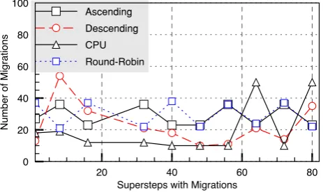
Figure 5.2 illustrates the number of migrations at each rescheduling call when considering α equal to 8. Considering the CPU strategy for initial scheduling, we can observe that MigCube selects a large number of processes to migrate at each attempt. The P M of the processes are closed to the largestP M, showing a large number of migrations at each rescheduling call. After analyzing the log of operations, we can observe a principle of hysteresis, i.e, several consecutive migrations in order to stabilize the behavior of the system. Moreover, in the current implementation, the migration test of a candidate process does not take into account the previous migration of other process to the same target (node or cluster), so contributing for the large number of observed migrations. These ideas explain the performance of the CPU strategy when compared to the remaining ones. Although obtaining good performance rates when comparing scenarios (i) and (iii), the CPU technique for initial scheduling achieves the worst performance among the other ones.
20 40 60 80 100 Number of Supersteps
0 10 20 30 40 50
Gain in Percentage
= 4 = 8 = 16
20 40 80 100
0 10 20 30 40 50
Gain in Percentage
= 4 = 8 = 16
20 40 60 80 100 Number of Supersteps
0 10 20 30 40 50
Gain in Percentage
= 4 = 8 = 16
20 40 60 80 100
Number of Supersteps 0 10 20 30 40 50
Gain in Percentage
= 4
= 8
= 16
(a) Ascending
60 Number of Supersteps
(b) Descending
(c) CPU (d) Round-Robin
∝
∝
∝
∝
∝
∝
∝
∝
∝
∝
∝
∝
Gain (%) Gain (%) Gain (%) Gain (%)Fig. 5.1: Percentage of gain in the execution time with MigCube-driven process rescheduling
20 40 60 80
Supersteps with Migrations 0 20 40 60 80 100
Number of Migrations
Ascending Descending
CPU
Round-Robin
Fig. 5.2: Number of migrations at each rescheduling call when using MigCube andα= 8.
efficient in the CPU perspective, the CPU initial mapping causes communication penalties because there are a large number of inter-cluster communication.
Table 5.2: MigHull evaluation. The times are expressed in seconds. We are highlighting the performance of scenario (i), where the CPU strategy for initial mapping presents large disparities
Supersteps
Scenarios
i ii iii ii iii ii iii
α= 4 α= 8 α= 16
Ascending
20 16.10 17.33 11.75 16.57 11.89 16.33 14.56
40 32.19 34.59 21.52 33.42 21.95 32.66 23.04
60 48.28 51.56 32.20 49.93 30.93 48.99 31.57
80 64.37 67.04 42.07 66.78 39.91 64.60 42.39
100 80.47 84.48 52.85 83.28 49.90 81.88 49.96
Descending
20 16.27 16.68 12.15 16.60 11.99 16.39 14.31
40 32.54 33.09 21.53 33.01 22.15 32.95 23.32
60 48.82 49.50 32.27 49.38 31.12 49.25 32.12
80 65.09 65.38 41.97 65.25 40.21 65.15 42.71
100 81.37 81.70 53.11 81.65 50.22 81.53 51.37
CPU
20 20.08 20.33 14.47 20.31 15.72 20.13 17.46
40 40.15 40.45 27.04 40.37 27.05 40.29 28.46
60 60.22 60.56 38.87 60.51 37.07 60.49 40.91
80 80.29 81.10 51.84 81.02 47.37 80.95 55.03
100 100.36 101.13 63.67 100.94 56.57 100.77 67.51
Round-Robin
20 16.16 17.11 11.61 16.42 11.81 16.30 14.50
40 32.33 34.12 21.20 33.01 21.93 32.49 23.04
60 48.46 51.13 31.85 49.29 30.87 48.68 31.97
80 64.56 65.15 41.44 65.89 39.87 65.09 43.20
100 80.60 83.60 52.10 82.17 49.85 81.20 50.70
MigHull strategy of using an intersection of the three 2D planes is responsible for reducing the number of migratable processes when compared to MigCube. Particularly, Figure 5.5 illustrates three moments of the execution for the Ascending strategy, showing the division of the processes among the clusters. We can observe the movement of the processes to take profit from the most powerful clusters, Chicon and Suno (see Section 4 for details regarding the subset of the Grid5000 infrastructure used in the tests).
5.3. MigCube and MigHull Comparative. Both MigCube and MigHull heuristics have the same objective and make use of the same idea: computational geometry to select a portion of process to migrate. Figure 5.6 illustrates the gains considering each initial scheduling and heuristic. The graph shows the mean value of gain of scenario (iii) over scenario (i) when considering all set of supersteps and α values. MigCube with the Ascending scheduling and αvalue equal to 4 achieved a gain of 25%, diverging significantly from the other results. This divergence occurs due to a low α, which makes many processes to migrate, increasing the communication between process and approximating metrics.
20 40 60 80 100 Number of Supersteps
0 10 20 30 40 50
Gain in Percentage
= 4
= 8
= 16
20 40 60 80 100
Number of Supersteps 0 10 20 30 40 50
Gain in Percentage
= 4
= 8
= 16
20 40 80 100
0 10 20 30 40 50
Gain in Percentage
= 4
= 8
= 16
20 40 60 80 100
Number of Supersteps 0 10 20 30 40 50
Gain in Percentage
= 4
= 8
= 16
(a) Ascending
60 Number of Supersteps
(b) Descending
(c) CPU (d) Round-Robin
∝
∝
∝
∝
∝
∝
∝
∝
∝
∝
∝
∝
Gain (%)Gain (%) Gain (%)
Gain (%)
Fig. 5.3: Percentage of gain in the execution time with MigHull-driven process rescheduling
20 40 60 80
Supersteps with Migrations 0 20 40 60 80 100
Number of Migrations
Ascending Descending CPU
Round-Robin
Fig. 5.4: Number of migrations at each rescheduling call when using MigHull andα= 8.
fourth migration call. Furthermore, we can observe that they achieved the main idea with process migration: to reduce the time of a superstep, so minimizing the application time as a whole.
Mapping at the begging of the execution
Mapping at superstep number 40
Mapping at the end of the execution
Fig. 5.5: Different moments of processes-clusters mappings when executing MigCube with the Ascending strat-egy for initial scheduling, 80 supersteps andα= 8.
5 10 15 20 25
Supersteps with Migrations 20
25 30 35 40 45
Gain in Percentage
MigCube-Ascending
MigCube-Descending
MigCube-CPU
MigCube-Round-Robin
MigHull-Ascending
MigHull-Descending
MigHull-CPU
MigHull-Round-Robin
Gain (%)
Fig. 5.6: Comparative involving MigCube and MigHull when varying the value ofα
MigHull come to fill the gap on process selection re-activity, not needing any intervention from the user nor previous knowledge about the BSP application.
Figure 5.8 shows a performance graph when considering the four aforementioned heuristics. This graph depicts, for each value of α, a mean value of the executions with the four initial scheduling. The gain refers to the performance of scenarios (i) and (iii). As expected, the heuristic that selects only one process obtained the worst results. The heuristic of percentage selection, that is using a 20% selection from the top PM has similar results to MigCube and MigHull. This happens because the percentage heuristic can select more process at each execution, providing a fast rescheduling of processes. The MigCube and MigHull achieve the best results due its analysis of each metric and the use of geometrical space.
20 40 60 80 Number of Supersteps
0 2 4 6 8 10 12 14
T
ime
Be
tw
e
e
n
Su
p
e
rst
e
p
s Without Migration
Migration with MigCube
Migration with MigHull
Fig. 5.7: Time between two supersteps in which migration calls took place.
0 10 20 30 40
Pe
rce
n
ta
g
e
o
f
G
a
in
∝
= 4∝
= 8∝
= 16
G
a
in
(%
)
MigCube
MigHull
Standard: 1 process
Standard: Percentage
Fig. 5.8: Comparing MigCube and MigHull with the standard MigBSP (approaches to select the migratable processes: only the process in the top of the PM list and a percentage of processes based on the top value of this list).
centralized and distributed strategies for load balancing. In the first one, all nodes send data about their CPU power and load to a master node. The master verifies the least and the most loaded node and migrates one process between them. In distributed approaches, every node choosesc(PUB parameter) other nodes randomly and asks them for their load. One process is migrated if the minimum load ofcanalyzed nodes is smaller than own load of the node that is performing the test.
Table 6.1: Related work comparison: F1 - Changing the application code; F2 - Platform: Grid or Cluster; F3 - Automatic selection of migratable processes,i.e., without user intervention; F4 - Use of computation metric (CPU load, CPU time or processing time) for load balancing; F5 - Use of communication data for load balancing; F6 Use of migration costs for load balancing; F7 Combination of metrics for load balancing purposes; F8 -Support for BSP applications; F9 - -Support of any kind of adaptivity on dynamic environments; F10 - -Support for heterogeneous systems; F11 - Process migration capability
Proposal Features
F1 F2 F3 F4 F5 F6 F7 F8 F9 F10 F11 MigBSP [28] No All No• Yes Yes Yes Yes Yes Yes Yes Yes HAMA [1] HDFS Cluster No No No No No Yes No Yes Yes PUB [7] No All Yes No No No Yes Yes Yes Yes Yes MulticoreBSP [37] Yes No NA† No No NA† No Yes No⋆ No⋆ No Mizan [19] No Cluster Yes No No No Yes Yes Yes Yes Yes BSPCloud [21] No Cluster No No No No Yes Yes Yes No Yes DistPM [20] No All Yes No No No Yes No Yes Yes Yes Pregel.NET [27] Yes Cloud Yes No No No No Yes Yes Yes Yes CPU-GPU cluster [24] Yes Cluster Yes No No No No Yes Yes Yes Yes References:•Depends on user definition at the beginning of the application;⋆Unknown;†Not Applicable.
Signal Processing) application implemented with the BSP computing model on a CPU-GPU cluster. During the processing phase of a BSP superstep, instead of moving the heavily loaded processes to another CPU, part of the load is divided to run in different GPUs. In this way, this middleware avoids network interaction, saving time on such operation. Unlike distributed systems, MulticoreBSP [37] library targets shared-memory computing employing thread-based parallelization. Finally, DistPM [20] is a library particularly developed to support process migration in grid computing. DistPM manages the network communication to avoid high data interaction between different clusters.
Table 6.1 summarizes the analysis of the aforementioned systems. We observe that our previous work named MigBSP is competitive among the BSP libraries regarding the load balancing perspective. Only MigBSP combines computation, communication and migration costs metrics for migration decision-making. Although having a process running in a slow processor that has a communication consistent pattern with a specific cluster, the migration penalties can act against migration viability, being dependent of process’ size and network characteristics. The MigBSP’s drawback considers how it selects the migratable processes, where now needs the intervention of user. In this way, both MigCube and MigHull proposed in this article seek to fill the MigBSP’s gap, which is being used today to run BSP-based weather forecast and oil prospection applications in the south of Brazil [30].
7. Conclusion. Considering that the bulk synchronous style is a common organization on writing success-ful parallel programs [7, 10, 17], MigCube and MigHull emerge as alternatives for selecting their processes for running on more suitable resources without interference from the users. The key contribution of the proposed heuristics is the efficient use of computation, communication and migration costs metrics as axes values in the computational geometry for process migration decision-making. As mentioned above, MigCube and MigHull are not restricted to the MigBSP’s scope, being employed to manage both heterogeneity and dynamism with process migration effortlessly at middleware level. Many data analysis techniques, such as machine learning and graph algorithms, require iterative computations and this is where Bulk Synchronous Parallel model can be more effective than MapReduce or Divide-and-Conquer strategies. The results showed gains larger than 40% when using MigCube or MigHull to decide process rescheduling in a subset of the Grid5000 environment. In addition, we also demonstrated a mean overhead close to 3% when employing the heuristics, but not perform-ing any migrations. The evaluation emphasized the capacity of both proposed heuristics with different initial processes-processors mappings over an heterogeneous cluster-based grid.
proposals on new complex applications including weather prediction and DNA sequencing [30]. Moreover, the use of a simulator was very convenient to evaluate the MigCube and MigHull feasibility. In this way, also as future work, we are analyzing communication libraries such as ProActive3 and AMPI4 to implement MigBSP
and the proposed heuristics. Consequently, real tests in the Grid5000 infrastructure will be conducted and compared with data obtained at simulation level.
Acknowledgements. This work was partially supported by the following Brazilian Agencies: CAPES, FAPERGS and CNPq.
REFERENCES
[1] Hama, June 2013. Available at: http://hama.apache.org/. Access: Jun. 2013. [2] Simgrid, June 2013. Available at: http://simgrid.gforge.inria.fr/. Access: Jun. 2013.
[3] V. Arabnejad, A. Moeini, and N. Moghadam, Using bee colony optimization to solve the task scheduling problem in homogenous systems, International Journal of Computer Science Issues, 8 (2011), pp. 348–353.
[4] S. Bandyapadhyay, S. Bhowmick, and K. Varadarajan,Approximation schemes for partitioning: Convex decomposition and surface approximation, in Proceedings of the Twenty-Sixth Annual ACM-SIAM Symposium on Discrete Algorithms, SODA ’15, SIAM, 2015, pp. 1457–1470.
[5] C. B. Barber, D. P. Dobkin, and H. Huhdanpaa,The quickhull algorithm for convex hulls, ACM Trans. Math. Softw., 22 (1996), pp. 469–483.
[6] M. d. Berg, O. Cheong, M. v. Kreveld, and M. Overmars, Computational Geometry: Algorithms and Applications, Springer-Verlag TELOS, Santa Clara, CA, USA, 3rd ed., 2008.
[7] O. Bonorden,Load Balancing in the Bulk-Synchronous-Parallel Setting using Process Migrations, 2007 IEEE International Parallel and Distributed Processing Symposium, (2007), pp. 1–9.
[8] O. Bonorden, B. Juurlink, I. von Otte, and I. Rieping,The paderborn university bsp (pub) library, Parallel Comput., 29 (2003), pp. 187–207.
[9] T. D. Braun, H. J. Siegel, N. Beck, L. L. B¨ol¨oni, M. Maheswaran, A. I. Reuther, J. P. Robertson, M. D. Theys, B. Yao, D. Hensgen, and R. F. Freund,A comparison of eleven static heuristics for mapping a class of independent tasks onto heterogeneous distributed computing systems, J. Parallel Distrib. Comput., 61 (2001), pp. 810–837.
[10] R. E. De Grande and A. Boukerche,Dynamic balancing of communication and computation load for hla-based simulations on large-scale distributed systems, J. Parallel Distrib. Comput., 71 (2011), pp. 40–52.
[11] G. El Kabbany, N. Wanas, N. Hegazi, and S. Shaheen,A dynamic load balancing framework for real-time applications in message passing systems, International Journal of Parallel Programming, 39 (2011), pp. 143–182.
[12] R. Fabbri, L. D. F. Costa, J. C. Torelli, and O. M. Bruno,2d euclidean distance transform algorithms: A comparative survey, ACM Comput. Surv., 40 (2008), pp. 2:1–2:44.
[13] Z. Fan, H. Shen, Y. Wu, and Y. Li,Simulated-annealing load balancing for resource allocation in cloud environments, in Proceedings of the 14th International Conference on Parallel and Distributed Computing, Applications and Technologies (PDCAT’13), New York, NY, USA, 2013, IEEE, pp. 1–6.
[14] V. Gaba and A. Prashar,Comparison of processor scheduling algorithms using genetic approach, International Journal of Advanced Research in Computer Science and Software Engineering, 2 (2012), pp. 37–45.
[15] M. R. Garey and D. S. Johnson,Computers and Intractability; A Guide to the Theory of NP-Completeness, W. H. Freeman & Co., New York, NY, USA, 1990.
[16] S. Hashemi and A. Hanani, Solving the scheduling problem in computational grid using artificial bee colony algorithm, Advances in Computer Science: an International Journal, 2 (2013), pp. 37–41.
[17] B. Hendrickson,Computational science: Emerging opportunities and challenges, Journal of Physics: Conference Series, 180 (2009), p. 012013.
[18] S. Kardani-Moghaddam, F. Khodadadi, R. Entezari-Maleki, and A. Movagha,A hybrid genetic algorithm and variable neighborhood search for task scheduling problem in grid environment, Procedia Engineering, 29 (2012), pp. 3808–3814. [19] Z. Khayyat, K. Awara, A. Alonazi, H. Jamjoom, D. Williams, and P. Kalnis, Mizan: a system for dynamic load
balancing in large-scale graph processing, in Proceedings of the 8th ACM European Conference on Computer Systems, EuroSys ’13, New York, NY, USA, 2013, ACM, pp. 169–182.
[20] Y. Li and Z. Lan,A novel workload migration scheme for heterogeneous distributed computing, in Cluster Computing and the Grid, 2005. CCGrid 2005. IEEE International Symposium on, vol. 2, 2005, pp. 1055–1062.
[21] X. Liu, W. Tong, and Y. Hou,BSPCloud: A Programming Model for Cloud Computing, 2012 IEEE 12th International Conference on Computer and Information Technology, (2012), pp. 1109–1113.
[22] A. Madureira, F. Santos, and I. Pereira,Self-managing agents for dynamic scheduling in manufacturing, in GECCO ’08: Proceedings of the 2008 GECCO conference companion on Genetic and evolutionary computation, New York, NY, USA, 2008, ACM, pp. 2187–2192.
[23] G. Malewicz, M. Austern, and A. Bik,Pregel: a system for large-scale graph processing, Proceedings of the 2010 ACM SIGMOD International Conference on Management of Data, (2010), pp. 135–145.
3
http://proactive.activeeon.com 4
[24] F. Mansouri, S. Huet, V. Fristot, and D. Houzet,Task migration of DSP application specified with a DFG and imple-mented with the BSP computing model on a CPU-GPU cluster, Proccedings of the 2013 Conf. on Design and Architectures for Signal and Image Processing (DASIP), IEEE, 2013, pp. 326-333.
[25] M. F. Pace,BSP vs mapreduce, Procedia Computer Science, 9 (2012), pp. 246 – 255. Proceedings of the International Conference on Computational Science, ICCS 2012.
[26] J. Pecero and P. Bouvry,An improved genetic algorithm for efficient scheduling on distributed memory parallel systems, in Proceedings of the International Conference on Computer Systems and Applications (AICCSA), New York, NY, USA, 2010, IEEE, pp. 1–8.
[27] M. Redekopp, Y. Simmhan, and V. Prasanna,Optimizations and analysis of bsp graph processing models on public clouds, in Parallel Distributed Processing (IPDPS), 2013 IEEE 27th International Symposium on, 2013, pp. 203–214.
[28] R. d. R. Righi, L. Graebin, and C. A. da Costa, On the replacement of objects from round-based applications over heterogeneous environments, Software: Practice and Experience, (2015), v. 45, n. 5, pp. 633-656.
[29] C. Schepke and N. Maillard, Performance improvement of the parallel lattice boltzmann method through blocked data distributions, in Computer Architecture and High Performance Computing, 2007. SBAC-PAD 2007. 19th International Symposium on, Oct 2007, pp. 71–78.
[30] J. Schneider, J. Gehr, H.-U. Heiss, T. Ferreto, C. De Rose, R. Righi, E. Rodrigues, N. Maillard, and P. Navaux, De-sign of a grid workflow for a climate application, in Computers and Communications, 2009. ISCC 2009. IEEE Symposium on, pp. 793–799.
[31] E.-G. Talbi,Metaheuristics : from design to implementation, John Wiley & Sons, Inc., Hoboken, NJ, USA, 2009.
[32] H. Tang, Y. Zhou, X. Huang, and G. Rong,Does pareto’s law apply to evidence distribution in software engineering? an initial report, in Proceedings of the 3rd International Workshop on Evidential Assessment of Software Technologies, EAST 2014, New York, NY, USA, 2014, ACM, pp. 9–16.
[33] L. G. Valiant,A bridging model for parallel computation, Commun. ACM, 33 (1990), pp. 103–111.
[34] H. Wu and C. Nie,An overview of search based combinatorial testing, in Proceedings of the 7th International Workshop on Search-Based Software Testing, SBST 2014, New York, NY, USA, 2014, ACM, pp. 27–30.
[35] A. Yzelman, R. Bisseling, D. Roose, and K. Meerbergen,Multicorebsp for c: A high-performance library for shared-memory parallel programming, International Journal of Parallel Programming, (2013), pp. 1–24.
[36] K. Ponnavaikko and J. Dharanipragada, Wide Area Distributed Filesystems - A Scalability and Performance Survey, Scalable Computing: Practice and Experience (SCPE), v.11, n.3, (2010), pp. 305-325.
[37] A. Yzelman and R. H. Bisseling,An object-oriented bulk synchronous parallel library for multicore programming, Concur-rency and Computation: Practice and Experience, 24 (2012), pp. 533–553.
[38] E. Cesario and D. Talia,Using Grids for Exploiting the Abundance of Data in Science, Scalable Computing: Practice and Experience (SCPE), v.11, n.3, (2010), pp. 251-261.